
Loading a real world dataset into ClickHouse often involves a journey through a number of simple steps. This post will be the first part in a series where we explore such datasets - in this case 1 billion rows of climate data from NOAA Global Historical Climatology Network - working through the typical process of sampling, preparing, enriching and loading the data before optimizing our schema for specific queries. We consider the exploration of datasets to be a key component of improving ClickHouse, not only for finding edge case issues, but to identify features that will make life easier for our users: we even track potential opportunities for fun with a specific GitHub label on the main repository.
This blog post originates from an issue created last year to explore the NOAA weather dataset. Various versions of this data exist in different formats and are of variable quality. Here we use a version distributed under awslabs that is a composite of climate records from numerous sources, merged, and subjected to a common suite of quality assurance reviews. We focus on cleansing and loading the data into ClickHouse before issuing some basic queries to confirm historical weather records, as well as more advanced features for inserting complementary datasets.
For our client machine, we use a c5ad.4xlarge with 16 cores and 32GB of RAM. ClickHouse is hosted on an AWS m5d.4xlarge instance with 16 cores and 64GB of RAM. We have also loaded this data into play.clickhouse.com for users to experiment and linked example queries where permissions permit.
Downloading the data
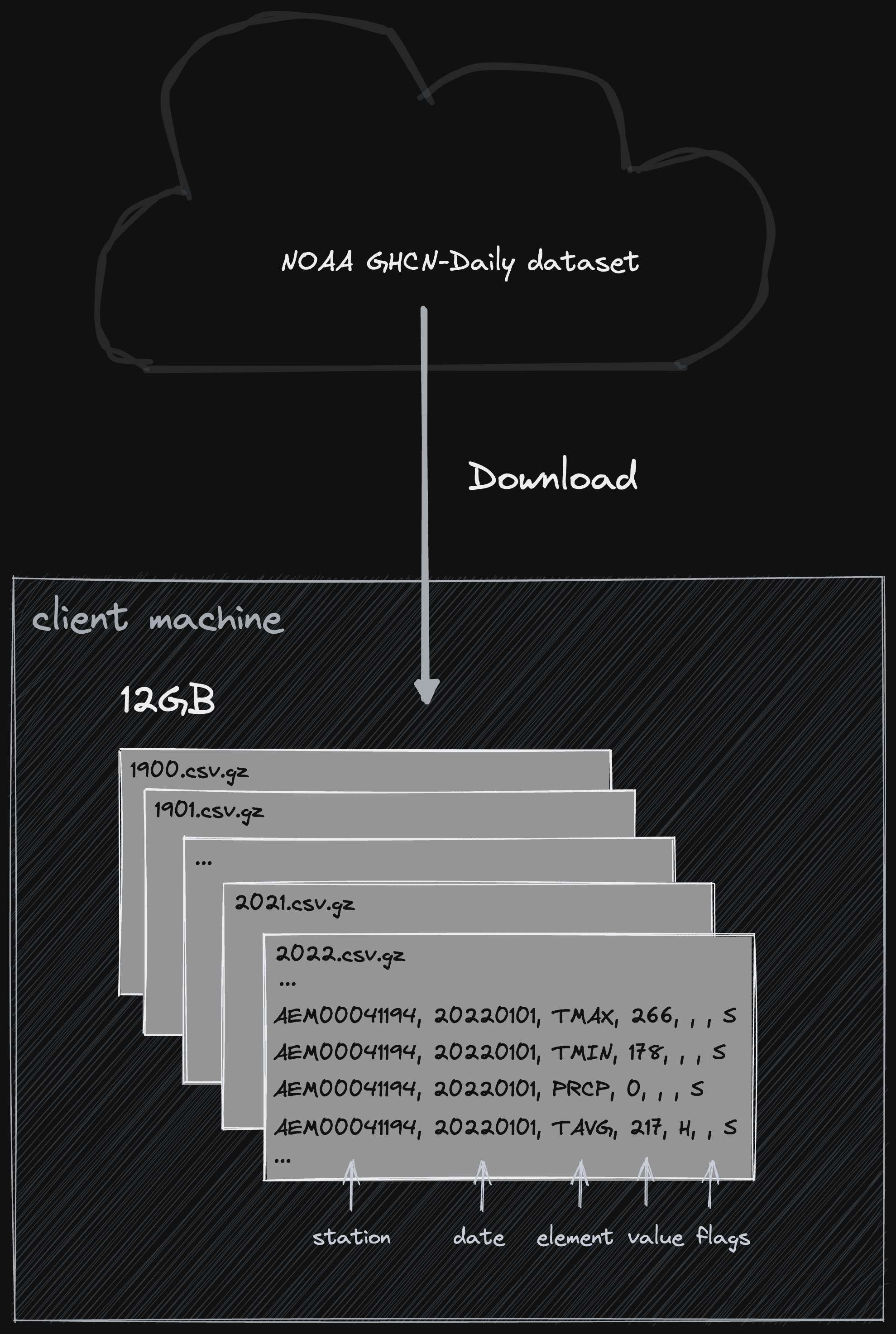
With ClickHouse recently adding support for dates from 1900, we can download the data from 1900 to 2022. If using an older version of ClickHouse, limit the range to 1925 - subsequent query results will thus obviously vary. The dataset is available in both csv and compressed gz. Since ClickHouse can read gz natively we prefer the latter since it's significantly smaller (12GB vs 100GB).
for i in {1900..2022}; do wget https://noaa-ghcn-pds.s3.amazonaws.com/csv.gz/${i}.csv.gz; done
Downloading this dataset takes around 10 mins, depending on your connection.
Sampling the data
In the past century, humans have dramatically increased their data collection efforts concerning the weather: The file representing the year 1900 has 4.6 million rows, while the 2022 file has almost 36 million. Sampling the data, we can see it distributed in a measurement per row format i.e.
zcat 2021.csv.gz | head
AE000041196,20210101,TMAX,278,,,S,
AE000041196,20210101,PRCP,0,D,,S,
AE000041196,20210101,TAVG,214,H,,S,
AEM00041194,20210101,TMAX,266,,,S,
AEM00041194,20210101,TMIN,178,,,S,
AEM00041194,20210101,PRCP,0,,,S,
AEM00041194,20210101,TAVG,217,H,,S,
AEM00041217,20210101,TMAX,262,,,S,
AEM00041217,20210101,TMIN,155,,,S,
AEM00041217,20210101,TAVG,202,H,,S,
Summarizing the format documentation and the columns in order:
- An 11 character station identification code. This itself encodes some useful information
- YEAR/MONTH/DAY = 8 character date in YYYYMMDD format (e.g. 19860529 = May 29, 1986)
- ELEMENT = 4 character indicator of element type. Effectively the measurement type. While there are many measurements available, we select the following:
- PRCP - Precipitation (tenths of mm)
- SNOW - Snowfall (mm)
- SNWD - Snow depth (mm)
- TMAX - Maximum temperature (tenths of degrees C)
- TAVG - Average temperature (tenths of a degrees C)
- TMIN - Minimum temperature (tenths of degrees C)
- PSUN - Daily percent of possible sunshine (percent)
- AWND - Average daily wind speed (tenths of meters per second)
- WSFG - Peak gust wind speed (tenths of meters per second)
- WT** = Weather Type where ** defines the weather type. Full list of weather types here.
- DATA VALUE = 5 character data value for ELEMENT i.e. the value of the measurement.
- M-FLAG = 1 character Measurement Flag. This has 10 possible values. Some of these values indicate questionable data accuracy. We accept data where this is set to “P” - identified as missing presumed zero, as this is only relevant to the PRCP, SNOW and SNWD measurements.
- Q-FLAG is the measurement quality flag with 14 possible values. We are only interested in data with an empty value i.e. it did not fail any quality assurance checks.
- S-FLAG is the source flag for the observation. Not useful for our analysis and ignored.
- OBS-TIME = 4-character time of observation in hour-minute format (i.e. 0700 =7:00 am). Typically not present in older data. We ignore this for our purposes.
Using clickhouse-local, a great tool allowing the processing of local files, we can filter rows that represent measurements of interest and pass our quality requirements, while avoiding the need to install and run ClickHouse.
clickhouse-local --query "SELECT count()
FROM file('*.csv.gz', CSV, 'station_id String, date String, measurement String, value Int64, mFlag String, qFlag String, sFlag String, obsTime String') WHERE qFlag = '' AND (measurement IN ('PRCP', 'SNOW', 'SNWD', 'TMAX', 'TAVG', 'TMIN', 'PSUN', 'AWND', 'WSFG') OR startsWith(measurement, 'WT'))"

2679255970
With over 2.6 billion rows, this isn’t a fast query since it involves parsing all the files. On our client machine, this takes around 160 seconds.
Note: the full dataset consists of 2,956,750,089 rows. We drop only 0.3% of rows by excluding those with quality challenges.
Preparing the data
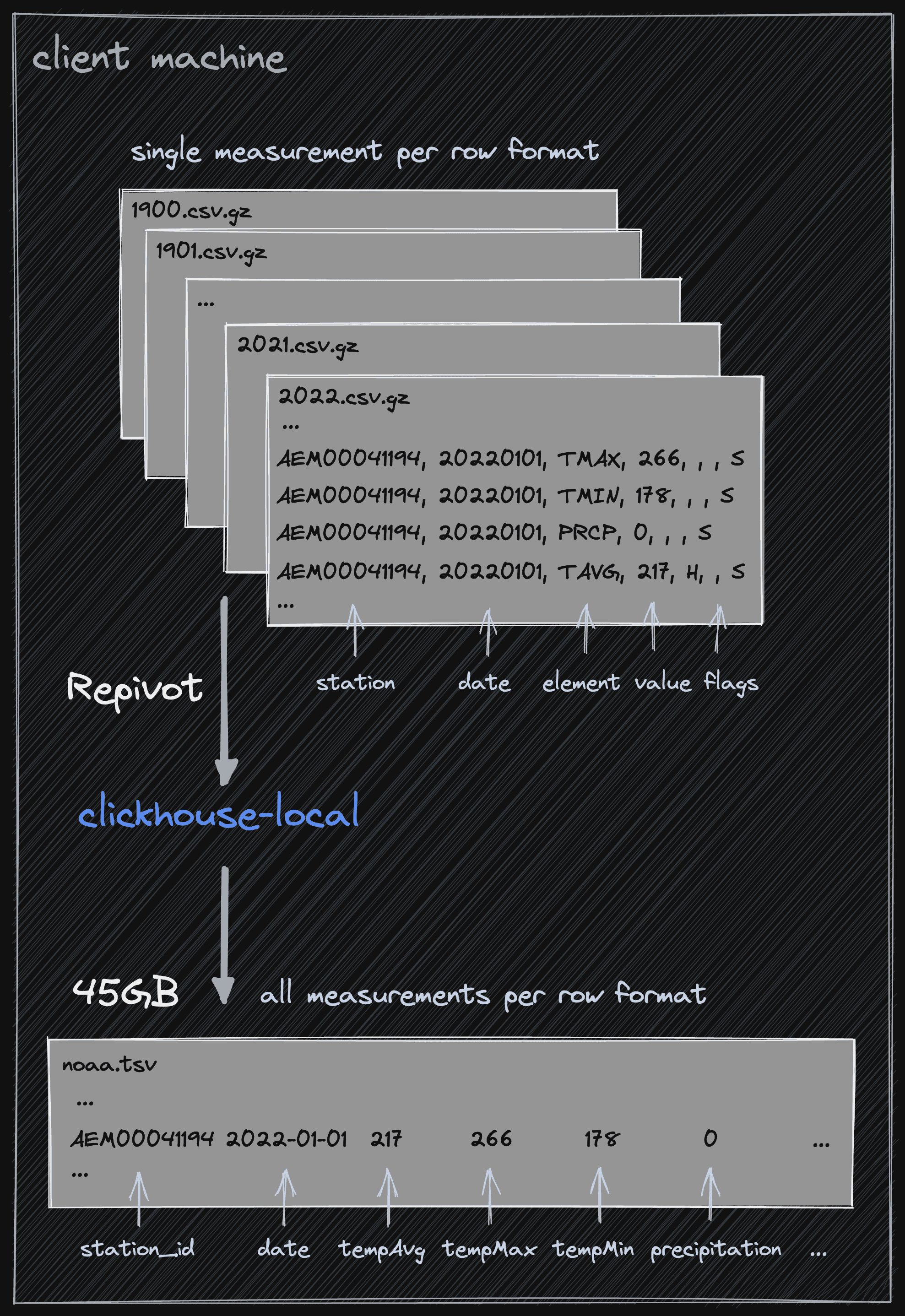
While the measurement per line structure can be used with ClickHouse, it will unnecessarily complicate future queries. Ideally, we need a row per station id and date, where each measurement type and associated value are a column i.e.
"station_id","date","tempAvg","tempMax","tempMin","precipitation","snowfall","snowDepth","percentDailySun","averageWindSpeed","maxWindSpeed","weatherType"
"AEM00041194","2022-07-30",347,0,308,0,0,0,0,0,0,0
"AEM00041194","2022-07-31",371,413,329,0,0,0,0,0,0,0
"AEM00041194","2022-08-01",384,427,357,0,0,0,0,0,0,0
"AEM00041194","2022-08-02",381,424,352,0,0,0,0,0,0,0
Using clickhouse-local and a simple GROUP BY we can repivot our data to this structure.
clickhouse-local --query "SELECT station_id,
       toDate32(date)  as date,
       anyIf(value, measurement = 'TAVG') as tempAvg,
       anyIf(value, measurement = 'TMAX') as tempMax,
       anyIf(value, measurement = 'TMIN') as tempMin,
       anyIf(value, measurement = 'PRCP') as precipitation,
       anyIf(value, measurement = 'SNOW') as snowfall,
       anyIf(value, measurement = 'SNWD') as snowDepth,
       anyIf(value, measurement = 'PSUN') as percentDailySun,
       anyIf(value, measurement = 'AWND') as averageWindSpeed,
       anyIf(value, measurement = 'WSFG') as maxWindSpeed,
       toUInt8OrZero(replaceOne(anyIf(measurement, startsWith(measurement, 'WT') AND value = 1), 'WT', '')) as weatherType
FROM file('./raw/*.csv.gz', CSV, 'station_id String, date String, measurement String, value Int64, mFlag String, qFlag String, sFlag String, obsTime String')
WHERE qFlag = ''
GROUP BY station_id, date
ORDER BY station_id, date FORMAT CSVWithNames;" > noaa.csv
This is a very memory intensive query. In the interest of performing this work on smaller machines, we can request that the aggregation overflow to disk with the max_bytes_before_external_group_by setting or simply compute a single file at a time:
for i in {1900..2022}
do
clickhouse-local --query "SELECT station_id,
       toDate32(date) as date,
       anyIf(value, measurement = 'TAVG') as tempAvg,
       anyIf(value, measurement = 'TMAX') as tempMax,
       anyIf(value, measurement = 'TMIN') as tempMin,
       anyIf(value, measurement = 'PRCP') as precipitation,
       anyIf(value, measurement = 'SNOW') as snowfall,
       anyIf(value, measurement = 'SNWD') as snowDepth,
       anyIf(value, measurement = 'PSUN') as percentDailySun,
       anyIf(value, measurement = 'AWND') as averageWindSpeed,
       anyIf(value, measurement = 'WSFG') as maxWindSpeed,
       toUInt8OrZero(replaceOne(anyIf(measurement, startsWith(measurement, 'WT') AND value = 1), 'WT', '')) as weatherType
FROM file('$i.csv.gz', CSV, 'station_id String, date String, measurement String, value Int64, mFlag String, qFlag String, sFlag String, obsTime String')
WHERE qFlag = ''
GROUP BY station_id, date
ORDER BY station_id, date FORMAT TSV" >> "noaa.tsv";
done
This query will take some time. To accelerate, we have several options: either parallelize by processing multiple files or load the data into a ClickHouse instance and utilize an INSERT SELECT to re-orientate the data as required. We explore the latter approach in "Final Enrichment".
Enriching the data
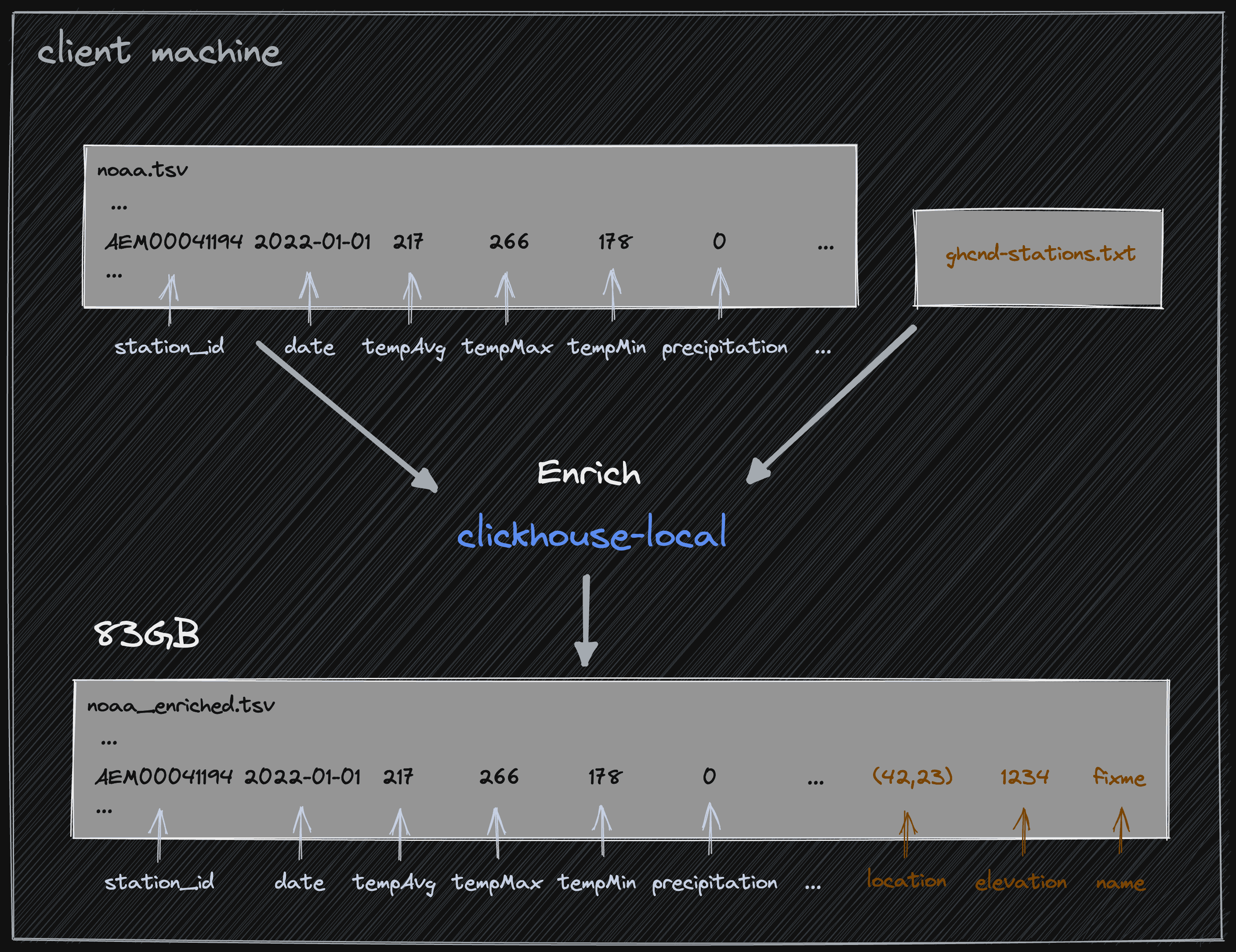
Our current data has no indication of location aside from a station id, which includes a prefix country code. Ideally, each station would have a latitude and longitude associated with it. To achieve this, NOAA conveniently provides the details of each station as a separate ghcnd-stations.txt. This file has several columns, of which five are useful to our future analysis: id, latitude, longitude, elevation, and name.
To parse this file, we use the Regexp Format with a simple regex group capturing each column. We join this to our newly created noaa.tsv.
wget http://noaa-ghcn-pds.s3.amazonaws.com/ghcnd-stations.txt
clickhouse-local --query "WITH stations AS (SELECT id, lat, lon, elevation, name FROM file('ghcnd-stations.txt', Regexp, 'id String, lat Float64, lon Float64, elevation Float32, name String'))
SELECT station_id,
       date,
       tempAvg,
       tempMax,
       tempMin,
       precipitation,
       snowfall,
       snowDepth,
       percentDailySun,
       averageWindSpeed,
       maxWindSpeed,
       weatherType,
       tuple(lon, lat) as location,
       elevation,
       name
FROM file('noaa.tsv', TSV,
          'station_id String, date Date32, tempAvg Int32, tempMax Int32, tempMin Int32, precipitation Int32, snowfall Int32, snowDepth Int32, percentDailySun Int8, averageWindSpeed Int32, maxWindSpeed Int32, weatherType UInt8') as noaa LEFT OUTER
         JOIN stations ON noaa.station_id = stations.id FORMAT TSV SETTINGS format_regexp='^(.{11})\s+(\-?\d{1,2}\.\d{4})\s+(\-?\d{1,3}\.\d{1,4})\s+(\-?\d*\.\d*)\s+(.*?)\s{2,}.*$'" > noaa_enriched.tsv
Note how we capture the longitude and latitude as a Point, represented as the tuple location. Our joined data is around 83GB.
Create our table
At just over a billion rows, this represents a fairly small dataset for ClickHouse, manageable by a single node and MergeTree table. Note to our users using ClickHouse Cloud - this DDL statement below will create a replicated merge tree transparently (the ENGINE can even be omitted). We will optimize the schema below in future blog posts and, for now, utilize a straightforward definition. The Enum allows us to capture the different types of weather events.
CREATE TABLE noaa
(
   `station_id` LowCardinality(String),
   `date` Date32,
   `tempAvg` Int32 COMMENT 'Average temperature (tenths of a degrees C)',
   `tempMax` Int32 COMMENT 'Maximum temperature (tenths of degrees C)',
   `tempMin` Int32 COMMENT 'Minimum temperature (tenths of degrees C)',
   `precipitation` UInt32 COMMENT 'Precipitation (tenths of mm)',
   `snowfall` UInt32 COMMENT 'Snowfall (mm)',
   `snowDepth` UInt32 COMMENT 'Snow depth (mm)',
   `percentDailySun` UInt8 COMMENT 'Daily percent of possible sunshine (percent)',
   `averageWindSpeed` UInt32 COMMENT 'Average daily wind speed (tenths of meters per second)',
   `maxWindSpeed` UInt32 COMMENT 'Peak gust wind speed (tenths of meters per second)',
   `weatherType` Enum8('Normal' = 0, 'Fog' = 1, 'Heavy Fog' = 2, 'Thunder' = 3, 'Small Hail' = 4, 'Hail' = 5, 'Glaze' = 6, 'Dust/Ash' = 7, 'Smoke/Haze' = 8, 'Blowing/Drifting Snow' = 9, 'Tornado' = 10, 'High Winds' = 11, 'Blowing Spray' = 12, 'Mist' = 13, 'Drizzle' = 14, 'Freezing Drizzle' = 15, 'Rain' = 16, 'Freezing Rain' = 17, 'Snow' = 18, 'Unknown Precipitation' = 19, 'Ground Fog' = 21, 'Freezing Fog' = 22),
   `location` Point,
   `elevation` Float32,
   `name` LowCardinality(String)
) ENGINE = MergeTree() ORDER BY (station_id, date);
Load the data
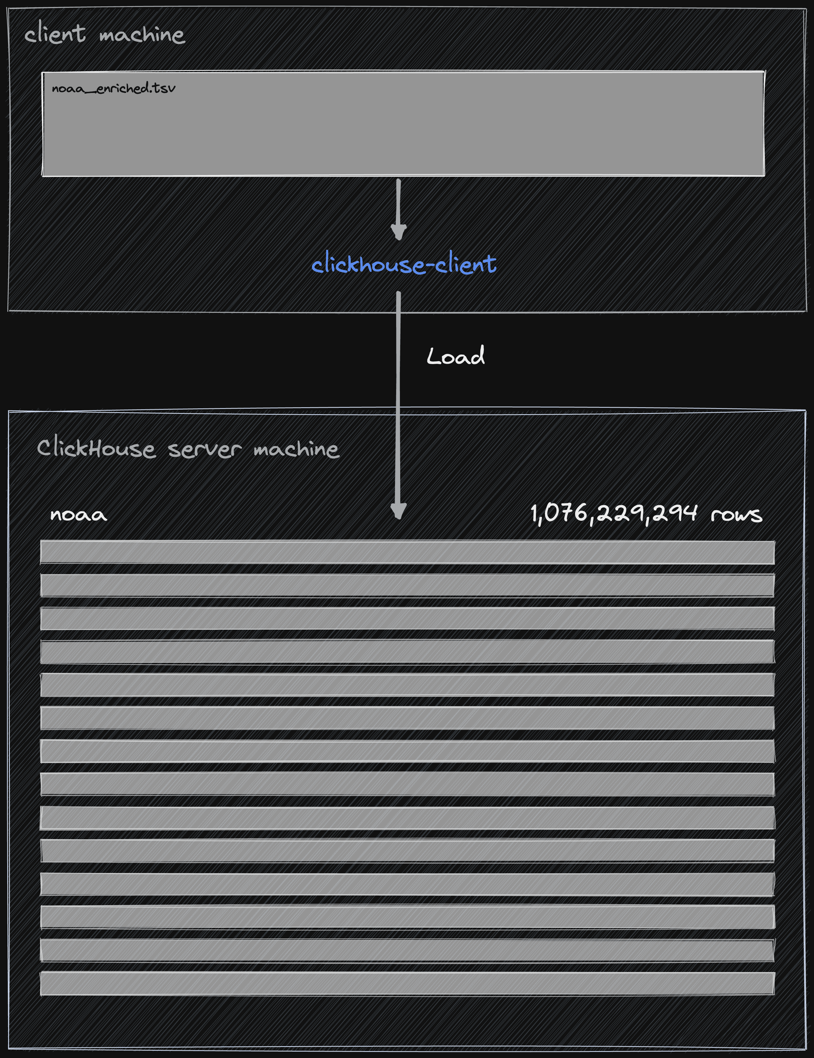
Previous efforts to pivot and clean the data ensure loading is now trivial. The simplest load method relies on the INFILE clause, which accepts a path to the local file for loading. We execute this within the clickhouse-client to ensure we receive details such as execution time and rows per second.
82GB in 195 seconds might seem a little slow to more experienced ClickHouse users. We can accelerate this in several ways, the quickest being to parallelize inserts. This requires us to split the files and invoke clickhouse-client for each. A full optimization task is beyond the scope here, but the following demonstrates splitting the file into 16 equal parts before invoking the client on each file in parallel.INSERT INTO noaa(station_id, date, tempAvg, tempMax, tempMin, precipitation, snowfall, snowDepth, percentDailySun, averageWindSpeed, maxWindSpeed, weatherType, location, elevation, name) FROM INFILE '/data/blog/noaa_enriched.tsv' FORMAT TSV; 1076229294 rows in set. Elapsed: 195.762 sec.
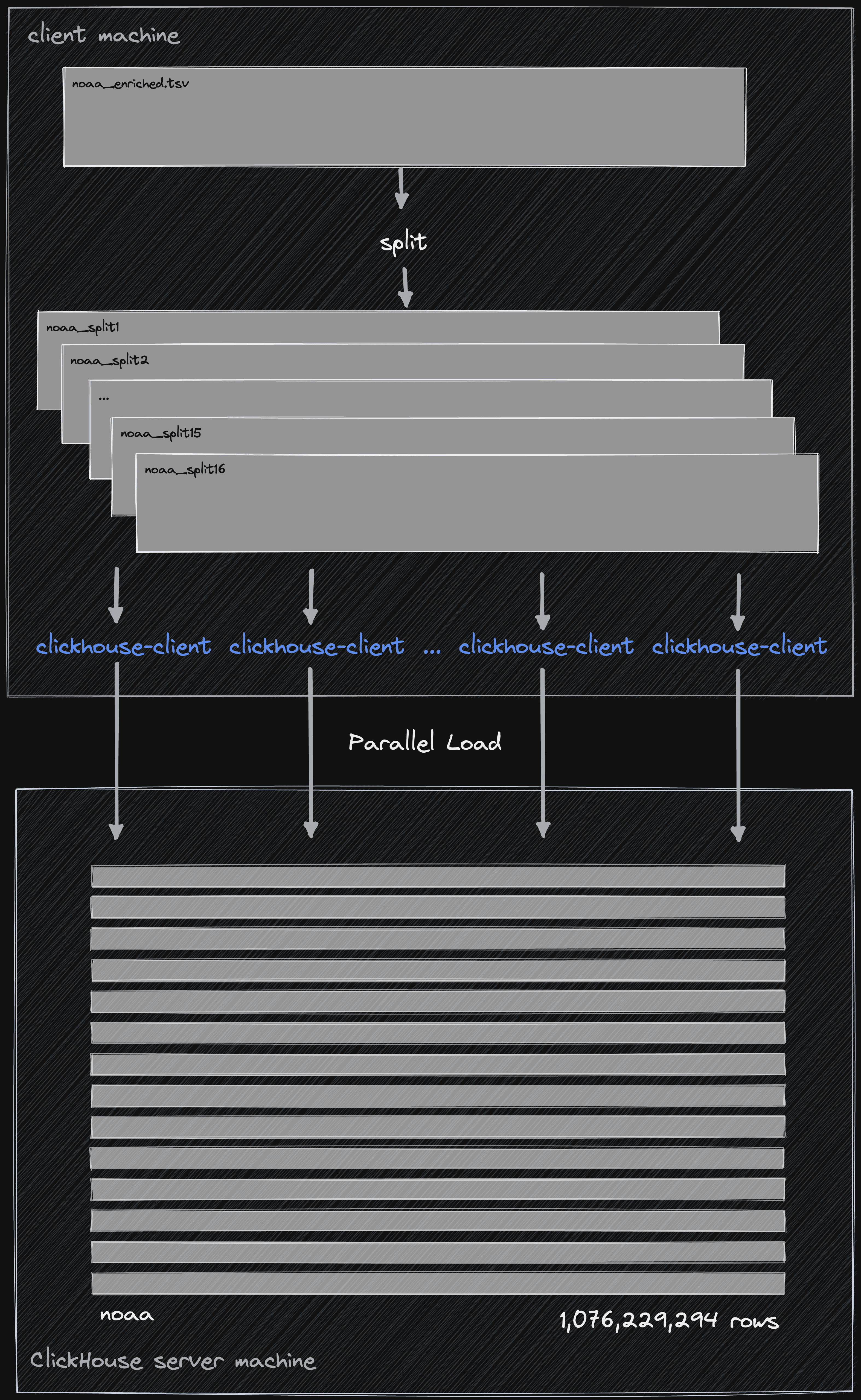
// split the file into roughly 16 equal parts
time split -l 67264331 noaa_enriched_2.tsv noaa_split

real    6m36.569s

// insert each file via clickhouse-client using a 16 separate process for each client
time find . -type f -name 'noaa_split*' | xargs -P 16 -n 1 -I {} sh -c "clickhouse-client --query 'INSERT INTO noaa(station_id, date, tempAvg, tempMax, tempMin, precipitation, snowfall, snowDepth, percentDailySun, averageWindSpeed, maxWindSpeed, weatherType, location, elevation, name) FORMAT TSV' < '{}'"

real    2m15.047s
This simple change, while probably not necessary, has reduced our load time down to 135 secs or around 620 mb/sec. For more technical readers, this is inline with the maximum read performance of our clients disks as measured by fio for a c5ad.4xlarge under a sequential read workload - based on steps here). Any gain here is offset by the time taken to split the files, so this approach only makes sense if your files are already in multiple parts. We could have generated multiple files in our enrichment step to later exploit this optimization.
Some Simple Queries
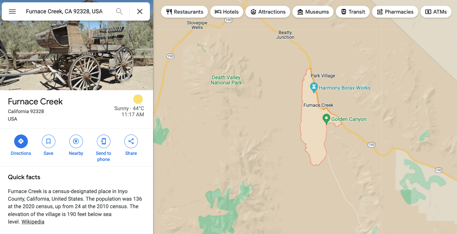
With the data loaded, we were keen to see how it compared to well-documented historical weather records. Although disputed, “according to the World Meteorological Organization (WMO), the highest temperature ever recorded was 56.7 °C (134.1 °F) on 10 July 1913 in Furnace Creek (Greenland Ranch), California, United States”.
Let's confirm this is the case with a trivial query - note we credit the first place to achieve a temperature (the dataset contains a few places achieving 56.7 since 1913) and filter to places where the temperature was recorded as being greater than 50C:
SELECT tempMax / 10 AS maxTemp, location, name, date FROM blogs.noaa WHERE tempMax > 500 ORDER BY tempMax DESC, date ASC LIMIT 5 ┌─maxTemp─┬─location──────────┬─name─────────────┬───────date─┐ │ 56.7 │ (-116.8667,36.45) │ CA GREENLAND RCH │ 1913-07-10 │ │ 56.7 │ (-115.4667,32.55) │ MEXICALI (SMN) │ 1949-08-20 │ │ 56.7 │ (-115.4667,32.55) │ MEXICALI (SMN) │ 1949-09-18 │ │ 56.7 │ (-115.4667,32.55) │ MEXICALI (SMN) │ 1952-07-17 │ │ 56.7 │ (-115.4667,32.55) │ MEXICALI (SMN) │ 1952-09-04 │ └─────────┴───────────────────┴──────────────────┴────────────┘ 5 rows in set. Elapsed: 0.107 sec. Processed 1.08 billion rows, 4.35 GB (10.03 billion rows/s., 40.60 GB/s.)✎
Reassuringly consistent with the documented record at Furnace Creek.
Final Enrichment
Any future, more complex weather analysis will likely need the ability to identify weather events for a specific geographical region. An area can theoretically be defined by a Polygon or even MultiPolygon (an array of Polygons) of lat/lon coordinates. The pointinpolygon query can be used to check if a weather event belongs to a polygon. We’ll use this feature in later blog posts for more interesting polygons, but for now, we will consider countries.
Datahub.io offers a number of useful smaller datasets, including a list of polygons for all countries of the world distributed as geojson. This allows us to demonstrate importing functions using the url function and performing data transformation at insert time.
This single JSON file contains the polygons of countries as elements of the array “features”. To obtain a row per country, with its respective polygon, we turn to the arrayJoin and JSONExtractArrayRaw functions.
SELECT arrayJoin(JSONExtractArrayRaw(json, 'features')) AS json
FROM url('https://datahub.io/core/geo-countries/r/0.geojson', JSONAsString)
LIMIT 1
FORMAT JSONEachRow

{"json":"{\"type\":\"Feature\",\"properties\":{\"ADMIN\":\"Aruba\",\"ISO_A3\":\"ABW\"},\"geometry\":{\"type\":\"Polygon\",\"coordinates\":[[[-69.99693762899992,12.577582098000036],[-69.93639075399994,12.53172435100005],[-69.92467200399994,12.519232489000046],[-69.91576087099992,12.497015692000076],[-69.88019771999984,12.453558661000045],[-69.87682044199994,12.427394924000097],[-69.88809160099993,12.417669989000046],[-69.90880286399994,12.417792059000107],[-69.93053137899989,12.425970770000035],[-69.94513912699992,12.44037506700009],[-69.92467200399994,12.44037506700009],[-69.92467200399994,12.447211005000014],[-69.95856686099992,12.463202216000099],[-70.02765865799992,12.522935289000088],[-70.04808508999989,12.53115469000008],[-70.05809485599988,12.537176825000088],[-70.06240800699987,12.546820380000057],[-70.06037350199995,12.556952216000113],[-70.0510961579999,12.574042059000064],[-70.04873613199993,12.583726304000024],[-70.05264238199993,12.600002346000053],[-70.05964107999992,12.614243882000054],[-70.06110592399997,12.625392971000068],[-70.04873613199993,12.632147528000104],[-70.00715084499987,12.5855166690001],[-69.99693762899992,12.577582098000036]]]}}"}
This still leaves us with one JSON blob per country. The fields indicating the country and its respective iso code are obvious: ADMIN and ISO_A3, respectively. Countries can either be Polygons when they are a single contiguous land area or MultiPolygons when they have complex land areas, e.g. Greece and its islands. Fortunately, the type field indicates which one is the case. To ensure future queries are simplified, we’ll convert all Polygons to MultiPolygons with some simple conditional logic. We use this statement inside an INSERT SELECT statement - a feature we’ve used in past posts, to insert the country data to a table.
CREATE TABLE countries
(
    `name` String,
    `coordinates` MultiPolygon
)
ENGINE = MergeTree
ORDER BY name

INSERT INTO countries SELECT
    name,
    coordinates
FROM
(
    SELECT
        JSONExtractString(JSONExtractString(json, 'properties'), 'ADMIN') AS name,
        JSONExtractString(JSONExtractRaw(json, 'geometry'), 'type') AS type,
        if(type = 'Polygon', [JSONExtract(JSONExtractRaw(JSONExtractRaw(json, 'geometry'), 'coordinates'), 'Polygon')], JSONExtract(JSONExtractRaw(JSONExtractRaw(json, 'geometry'), 'coordinates'), 'MultiPolygon')) AS coordinates
    FROM
    (
        SELECT arrayJoin(JSONExtractArrayRaw(json, 'features')) AS json
        FROM url('https://datahub.io/core/geo-countries/r/0.geojson', JSONAsString)
    )
)
With this supplementary dataset we can use the pointInPolygon function to identify the weather events that occur within the polygons of a country, Portugal. Note how we have to iterate through the polygons of the multi-polygon field using arrayExists. Portugal itself has 17 polygons to capture its boundaries - the result is that this many comparisons are required per weather event to find the hottest day on record.
WITH (
      SELECT coordinates
      FROM countries
      WHERE name = 'Portugal'
  ) AS pCoords
SELECT
    tempMax,
    station_id,
    date,
    location
FROM noaa
WHERE arrayExists(cord -> pointInPolygon(location, cord), pCoords)
ORDER BY tempMax DESC
LIMIT 5

┌─tempMax─┬─station_id──┬───────date─┬─location──────────┐
│     458 │ PO000008549 │ 1944-07-30 │ (-8.4167,40.2)    │
│     454 │ PO000008562 │ 2003-08-01 │ (-7.8667,38.0167) │
│     452 │ PO000008562 │ 1995-07-23 │ (-7.8667,38.0167) │
│     445 │ POM00008558 │ 2003-08-01 │ (-7.9,38.533)     │
│     442 │ POM00008558 │ 2022-07-13 │ (-7.9,38.533)     │
└─────────┴─────────────┴────────────┴───────────────────┘

10 rows in set. Elapsed: 3388.576 sec. Processed 1.06 billion rows, 46.83 GB (314.06 thousand rows/s., 13.82 MB/s.
While the response is consistent with Portugal’s historical records, this query is very slow at nearly an hour. For more elaborate countries, e.g. Canada, this query would be unviable.
SELECT
   name,
   length(coordinates) AS num_coordinates
FROM countries
ORDER BY num_coordinates DESC
LIMIT 5

┌─name─────────────────────┬─num_coordinates─┐
│ Canada                   │             410 │
│ United States of America │             346 │
│ Indonesia                │             264 │
│ Russia                   │             213 │
│ Antarctica               │             179 │
└──────────────────────────┴─────────────────┘
To accelerate this query, we can use Polygon dictionaries. These allow users to search for the polygon containing specified points efficiently. We largely use the defaults to define our dictionary, using the countries table as its source.
Our query subsequently becomes:CREATE DICTIONARY country_polygons ( `name` String, `coordinates` MultiPolygon ) PRIMARY KEY coordinates SOURCE(CLICKHOUSE(TABLE 'countries')) LIFETIME(MIN 0 MAX 0) LAYOUT(POLYGON(STORE_POLYGON_KEY_COLUMN 1))
That's better*! And for the worst case Canada?SELECT tempMax / 10 AS maxTemp, station_id, date, location FROM noaa WHERE dictGet(country_polygons, 'name', location) = 'Portugal' ORDER BY tempMax DESC LIMIT 5✎Query id: bfb88bc1-4c1d-4808-bd2d-3a2406d387c3
┌─maxTemp─┬─station_id──┬───────date─┬─location──────────┐ │ 45.8 │ PO000008549 │ 1944-07-30 │ (-8.4167,40.2) │ │ 45.4 │ PO000008562 │ 2003-08-01 │ (-7.8667,38.0167) │ │ 45.2 │ PO000008562 │ 1995-07-23 │ (-7.8667,38.0167) │ │ 44.5 │ POM00008558 │ 2003-08-01 │ (-7.9,38.533) │ │ 44.2 │ POM00008558 │ 2022-07-13 │ (-7.9,38.533) │ └─────────┴─────────────┴────────────┴───────────────────┘
5 rows in set. Elapsed: 14.498 sec. Processed 1.06 billion rows, 46.83 GB (73.40 million rows/s., 3.23 GB/s.)
*Note the first time this query is issued, the dictionary will be loaded into memory - this takes around 5s. Subsequent queries should be consistent. To load the dictionary with a trivial query, we can issue a simple dictGet. e.g.
SELECT dictGet(country_polygons, 'name', (-9.3704, 38.8027));
SELECT tempMax / 10 AS maxTemp, station_id, date, location FROM noaa WHERE dictGet(country_polygons, 'name', location) = 'Canada' ORDER BY tempMax DESC LIMIT 5 ┌─maxTemp─┬─station_id──┬───────date─┬─location───────┐ │ 47.3 │ CA001163780 │ 2021-06-30 │ (-120.45,50.7) │ │ 46.6 │ CA001163780 │ 2021-07-01 │ (-120.45,50.7) │ │ 46.2 │ CA001163842 │ 2021-06-30 │ (-120.45,50.7) │ │ 45.3 │ CA001163842 │ 2021-07-01 │ (-120.45,50.7) │ │ 45 │ CA004015160 │ 1937-07-05 │ (-103.4,49.4) │ └─────────┴─────────────┴────────────┴────────────────┘ 5 rows in set. Elapsed: 14.481 sec. Processed 1.06 billion rows, 46.83 GB (73.49 million rows/s., 3.23 GB/s.)✎
Similar performance and independent of the polygon complexity! also consistent with Canada’s record - although the location and exact temperature are slightly off.
On implementing this particular query, it became apparent that the first two letters of the station_id represent the country - a lesson in knowing your data. A simpler (and faster) equivalent query to the above is shown below. Polygon Dictionaries do offer a more flexible solution, however, in that they allow us to potentially match arbitrary land areas.
Finally, as an avid skier, I was personally curious about the best place to have skied in the United States in the last 5 yrs.SELECT tempMax / 10 AS maxTemp, station_id, date, location FROM noaa WHERE substring(station_id, 1, 2) = 'CA' ORDER BY tempMax DESC LIMIT 5 ┌─maxTemp─┬─station_id──┬───────date─┬─location───────┐ │ 47.3 │ CA001163780 │ 2021-06-30 │ (-120.45,50.7) │ │ 46.6 │ CA001163780 │ 2021-07-01 │ (-120.45,50.7) │ │ 46.2 │ CA001163842 │ 2021-06-30 │ (-120.45,50.7) │ │ 45.3 │ CA001163842 │ 2021-07-01 │ (-120.45,50.7) │ │ 45 │ CA004015160 │ 1937-07-05 │ (-103.4,49.4) │ └─────────┴─────────────┴────────────┴────────────────┘ 5 rows in set. Elapsed: 3.000 sec. Processed 1.06 billion rows, 22.71 GB (354.76 million rows/s., 7.57 GB/s.)✎
Using a list of ski resorts in the united states and their respective locations, we join these against the top 1000 weather stations with the most in any month in the last 5 yrs. Sorting this join by geoDistance and restricting the results to those where the distance is less than 20km, we select the top result per resort and sort this by total snow. Note we also restrict resorts to those above 1800m, as a broad indicator of good skiing conditions.
Please don’t use the results as advice for planning your future holiday destinations, not least because altitude and volume of snow != quality of skiing.SELECT resort_name, total_snow / 1000 AS total_snow_m, resort_location, month_year FROM ( WITH resorts AS ( SELECT resort_name, state, (lon, lat) AS resort_location, 'US' AS code FROM url('https://gist.githubusercontent.com/Ewiseman/b251e5eaf70ca52a4b9b10dce9e635a4/raw/9f0100fe14169a058c451380edca3bda24d3f673/ski_resort_stats.csv', CSVWithNames) ) SELECT resort_name, highest_snow.station_id, geoDistance(resort_location.1, resort_location.2, station_location.1, station_location.2) / 1000 AS distance_km, highest_snow.total_snow, resort_location, station_location, month_year FROM ( SELECT sum(snowfall) AS total_snow, station_id, any(location) AS station_location, month_year, substring(station_id, 1, 2) AS code FROM noaa WHERE (date > '2017-01-01') AND (code = 'US') AND (elevation > 1800) GROUP BY station_id, toYYYYMM(date) AS month_year ORDER BY total_snow DESC LIMIT 1000 ) AS highest_snow INNER JOIN resorts ON highest_snow.code = resorts.code WHERE distance_km < 20 ORDER BY resort_name ASC, total_snow DESC LIMIT 1 BY resort_name, station_id ) ORDER BY total_snow DESC LIMIT 5 ┌─resort_name──────────┬─total_snow_m─┬─resort_location─┬─month_year─┐ │ Sugar Bowl, CA │ 7.799 │ (-120.3,39.27) │ 201902 │ │ Donner Ski Ranch, CA │ 7.799 │ (-120.34,39.31) │ 201902 │ │ Boreal, CA │ 7.799 │ (-120.35,39.33) │ 201902 │ │ Homewood, CA │ 4.926 │ (-120.17,39.08) │ 201902 │ │ Alpine Meadows, CA │ 4.926 │ (-120.22,39.17) │ 201902 │ └──────────────────────┴──────────────┴─────────────────┴────────────┘ 5 rows in set. Elapsed: 2.119 sec. Processed 989.55 million rows, 24.99 GB (467.07 million rows/s., 11.80 GB/s.)
In the next post in this series we’ll delve into this dataset in more detail and try to answer some more interesting questions, as well explore some visualization techniques for geo data.
Acknowledgments
We would like to acknowledge the efforts of the Global Historical Climatology Network for preparing, cleansing, and distributing this data. We appreciate your efforts.
Menne, M.J., I. Durre, B. Korzeniewski, S. McNeal, K. Thomas, X. Yin, S. Anthony, R. Ray, R.S. Vose, B.E.Gleason, and T.G. Houston, 2012: Global Historical Climatology Network - Daily (GHCN-Daily), Version 3. [indicate subset used following decimal, e.g. Version 3.25]. NOAA National Centers for Environmental Information. http://doi.org/10.7289/V5D21VHZ [17/08/2020]