
This blog post is part of a series:
This post continues the series "Getting Data Into ClickHouse". In our previous post, we showed the basics of loading a Hacker News dataset and took a small detour into the world of JSON. In this post, we continue exploring ways to get data into ClickHouse, focusing on using Amazon S3 storage as both a source of data and as a queryable data repository in its own right. For this post, we’ll also explore a new dataset: foreign exchange (“forex”) data from the last 20 yrs. This has a trivial schema but is useful in its properties and lets us explore window functions.
Amazon S3 or Amazon Simple Storage Service is a service offered by Amazon Web Services that provides object storage through a web service interface. In the last 10 years, it has become almost ubiquitous as both a storage layer for data (see ClickHouse Cloud) and as a means of file distribution. We increasingly encounter ClickHouse users who have used S3 as a data lake and wish to either import this data into ClickHouse or query the data in place. This post shows how both approaches can be achieved using ClickHouse.
While our examples use ClickHouse Cloud, these should apply to self-managed instances and runnable on any moderate laptop.
A little bit about forex...
This blog post isn’t about forex trading, which can be an involved topic and involve some complex strategies! However, to give users some context for future ClickHouse queries and a basic understanding of the data, we briefly explain the core concepts. Understanding forex trading is not mandatory to be able to follow the technical aspects in this post, but will help explain the motivations behind the queries.
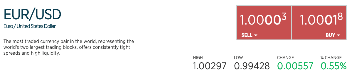
Forex trading is the trading of currencies from different countries against each other; for example, the US Dollar against the Euro. Any currency trade occurs between a pair of currencies. The purchasing of a currency pair involves two parties, such as a trader and a broker. The trader can either buy a base currency with a quote currency from the broker or sell a base currency and receive the quote in return. This pair is quoted in the format X/Y, where X is the base and Y is the quote. For example, the sample data below shows the bid and quote prices for the pair EUR/USD (a major pair) in 2022.
Given the above, the ask quote (or ask price) represents the price the broker is willing to accept in quote currency for every unit of the base currency they are selling, i.e., it is what they are asking for. This is what the trader can open a BUY position at.
The bid quote (or bid/offer price) is what the broker is willing to buy or BID in quote currency for the base currency. The trader opens a SELL (short) position at this price.
The ask quote will always be higher than the bid quote. The trader will always pay more for the pair than what they can get back. The difference between the bid and ask is the spread and is effectively the margin for the broker and how institutions make money.
For example, consider the following quote for the EUR/USD pair from 02/09/2022 from forex.com.
Pips and Ticks
The minimum unit of measurement when trading a currency pair is the Point in Price or PiP. This is typically the 4th decimal place for most major currency pairs or, in some cases, the 2nd, e.g., for pairs involving the Japanese yen. A currency pair’s prices are, in turn, usually measured one decimal place higher. Note that spreads are also measured in pips.
Ticks record when the price of a stock or commodity changes by a predetermined amount or fractional change, i.e., a tick occurs when the price moves up or down by a specific amount or fractional change. In forex, a tick will happen when either the bid or quote price changes by a pip of the currency pair.
The Data
The dataset used in this blog post was downloaded from www.histdata.com. The dataset consists of around 11.5 billion rows/ticks and is almost 600GB decompressed, with a total of 66 currency pairs. It covers the period May 2000 to August 2022 but is not equally distributed over this period, i.e., there are significantly more ticks in later years than in 2000, as we’ll later illustrate. This is likely more a factor of data availability than market activity, and the fact collection was only “best effort.” As a result, the volume of rows for any currency is likely not a good indicator of trading activity.
We provide a cleaned version of the tick data for ClickHouse testing. Users looking to obtain a more recent version of the data, or continuous updates, should consult www.histdata.com, which provides paid updates for a nominal fee in various formats.
The original data comes in a few variants, documented here. We specifically focus on the Ascii tick data that provides the highest level of granularity. In this post, we’ll focus on using a clean version of the data and skip the download and preparation steps. For those interested, we have documented the steps to download and cleanse this dataset here.
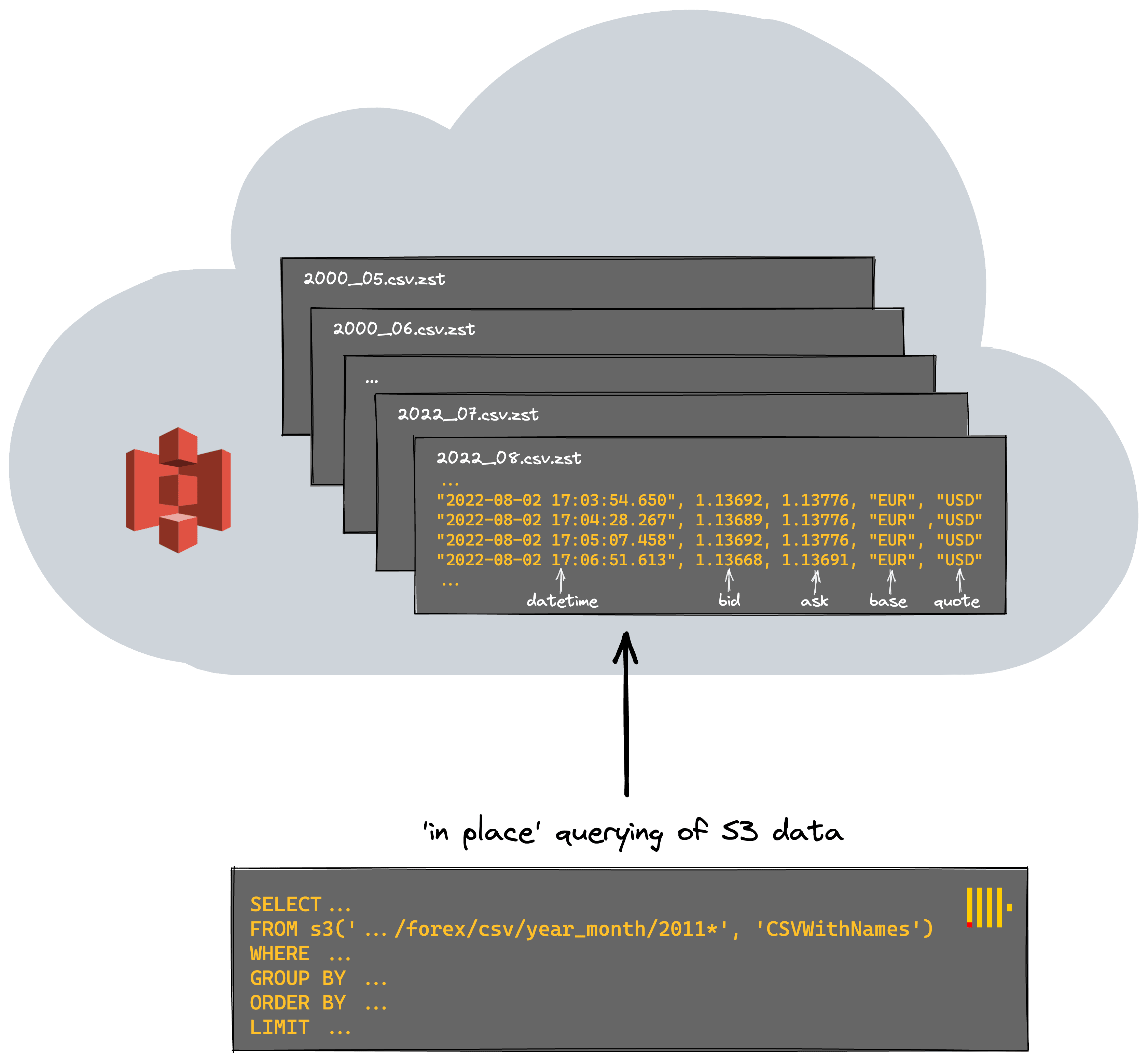
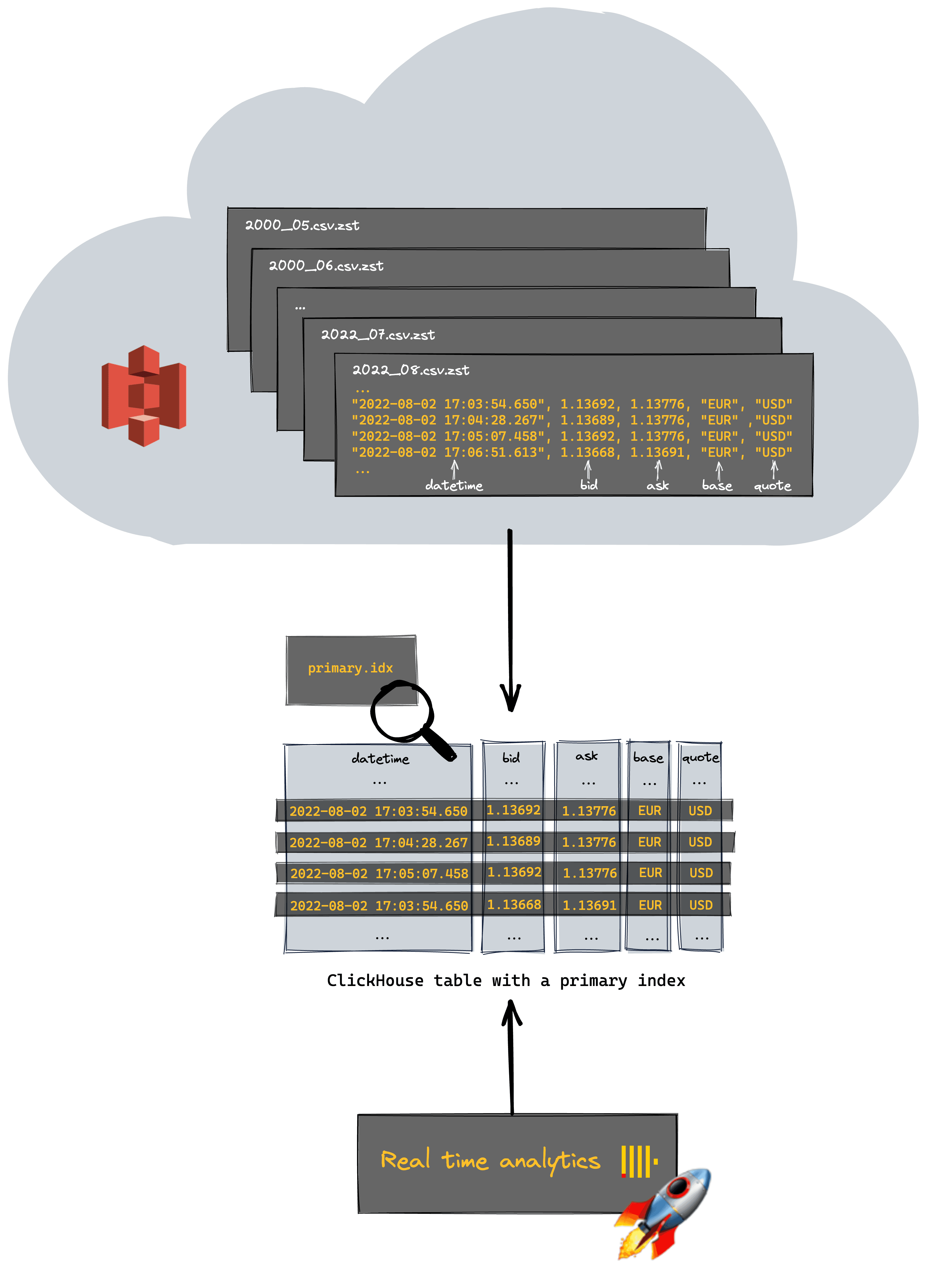
Our processed data consists of 5 columns, with a row per tick, containing the time to ms granularity, an indication of base and quote currency and the ask and bid quotes.
"datetime","bid","ask","base","quote"
"2022-01-02 17:03:54.650",1.1369,1.13776,"EUR","USD"
"2022-01-02 17:04:28.267",1.13689,1.13776,"EUR","USD"
"2022-01-02 17:05:07.458",1.13692,1.13776,"EUR","USD"
"2022-01-02 17:06:51.613",1.13668,1.1369,"EUR","USD"
It is important to emphasize that the tick data does not represent an actual trade/exchange. The number of trades/exchanges per second is significantly higher than a few per second! Nor does it capture the price that was agreed or the volume of the currency which was exchanged (logically 0 in the source data and hence ignored). Rather it simply marks when the bid or quote price is changed by a pip for the currency pair.
The data itself is distributed in 2 formats: zst compressed csv and parquet. Each set provides a file per month/year, resulting in 269 files for each. These sets are located under the S3 buckets s3://datasets-documentation/forex/parquet/year_month and s3://datasets-documentation/forex/csv/year_month/.
Querying data in place
For frequently accessed datasets, it is a good idea to load them into an analytical database like ClickHouse, so you can query it very fast. But for infrequently used datasets, it’s sometimes useful to leave them in a “data lake” like S3 and have the ability to run ad-hoc analytical queries on them in place. In the AWS ecosystem, users may be familiar with technologies such as Amazon Athena, which offers the ability to analyze data directly in Amazon S3 using standard SQL. However, to query data from structured tables, users would have to also use an analytical data warehouse like Redshift, and switch between those two tools.
ClickHouse solves both of these requirements with a single technology, simplifying usage and allowing users to select the appropriate approach with a function choice. Need an optimized table format with unparalleled query speed? ClickHouse provides various ways to structure the data (e.g. the MergeTree family table engine) for fast queries. Need to query data in place? For datasets for which infrequent analysis is required, ClickHouse offers the ability to query data directly in external tables S3 using functions such as the S3 table function as shown below.
Below we compute the number of ticks per currency pair for 2021. Note how we are able to restrict the files using a glob pattern.
SELECT
    base,
    quote,
    count() AS total
FROM s3('https://datasets-documentation.s3.eu-west-3.amazonaws.com/forex/csv/year_month/2011*', 'CSVWithNames')
GROUP BY
    base,
    quote
LIMIT 10
FORMAT PrettyMonoBlock
┏━━━━━━┳━━━━━━━┳━━━━━━━━━━┓
┃ base ┃ quote ┃    total ┃
┡━━━━━━╇━━━━━━━╇━━━━━━━━━━┩
│ EUR  │ NOK   │  3088787 │
├──────┼───────┼──────────┤
│ USD  │ JPY   │  1920648 │
├──────┼───────┼──────────┤
│ USD  │ TRY   │  2442707 │
├──────┼───────┼──────────┤
│ XAU  │ USD   │ 10529876 │
├──────┼───────┼──────────┤
│ USD  │ CAD   │  3264491 │
├──────┼───────┼──────────┤
│ EUR  │ PLN   │  1840402 │
├──────┼───────┼──────────┤
│ EUR  │ AUD   │  8072459 │
├──────┼───────┼──────────┤
│ GRX  │ EUR   │  8558052 │
├──────┼───────┼──────────┤
│ CAD  │ JPY   │  5598892 │
├──────┼───────┼──────────┤
│ BCO  │ USD   │  5620577 │
└──────┴───────┴──────────┘

10 rows in set. Elapsed: 26.290 sec. Processed 423.26 million rows, 11.00 GB (16.10 million rows/s., 418.59 MB/s.)
Ticks are not the best indicator of market activity. The most commonly traded pairs, however, will have the highest liquidity - under normal market conditions, which is typically expressed as a low spread. As a reminder, the spread is the difference between the ask and bid price. Let's compute this for the entire dataset over all pairs. We rely on schema inference to avoid any specification of the schema.
SELECT
    base,
    quote,
    avg(ask - bid) AS spread
FROM s3('https://datasets-documentation.s3.eu-west-3.amazonaws.com/forex/csv/year_month/*.csv.zst', 'CSVWithNames')
GROUP BY
    base,
    quote
ORDER BY spread ASC
LIMIT 10

┌─base─┬─quote─┬─────────────────spread─┐
│ EUR  │ USD   │ 0.00009969029669160744 │
│ EUR  │ GBP   │ 0.00013673935811218818 │
│ AUD  │ USD   │ 0.00015432083736303172 │
│ NZD  │ USD   │  0.0001697723724941787 │
│ EUR  │ CHF   │  0.0001715531048879742 │
│ USD  │ CAD   │ 0.00017623255399539916 │
│ GBP  │ USD   │ 0.00019109680654318212 │
│ USD  │ SGD   │ 0.00021710273761740704 │
│ USD  │ CHF   │ 0.00021764358513112766 │
│ CAD  │ CHF   │  0.0002664969070414096 │
└──────┴───────┴────────────────────────┘

10 rows in set. Elapsed: 582.913 sec. Processed 11.58 billion rows, 509.59 GB (19.87 million rows/s., 874.21 MB/s.)
This doesn't fully correlate with the most popular currency pairs, mainly as some currencies use a two-decimal pip. While possibly an unrealistic query across the entire dataset, we've processed 11.58GB of data and obtained a result in under 10 minutes at almost 20m rows/sec. Users running this command might notice that our throughput continuously increases. This is a property of the data - later months have more data and are larger files, thus benefiting more from parallelization. Let's see if we do better than this before trying some more interesting queries.
Speeding things up
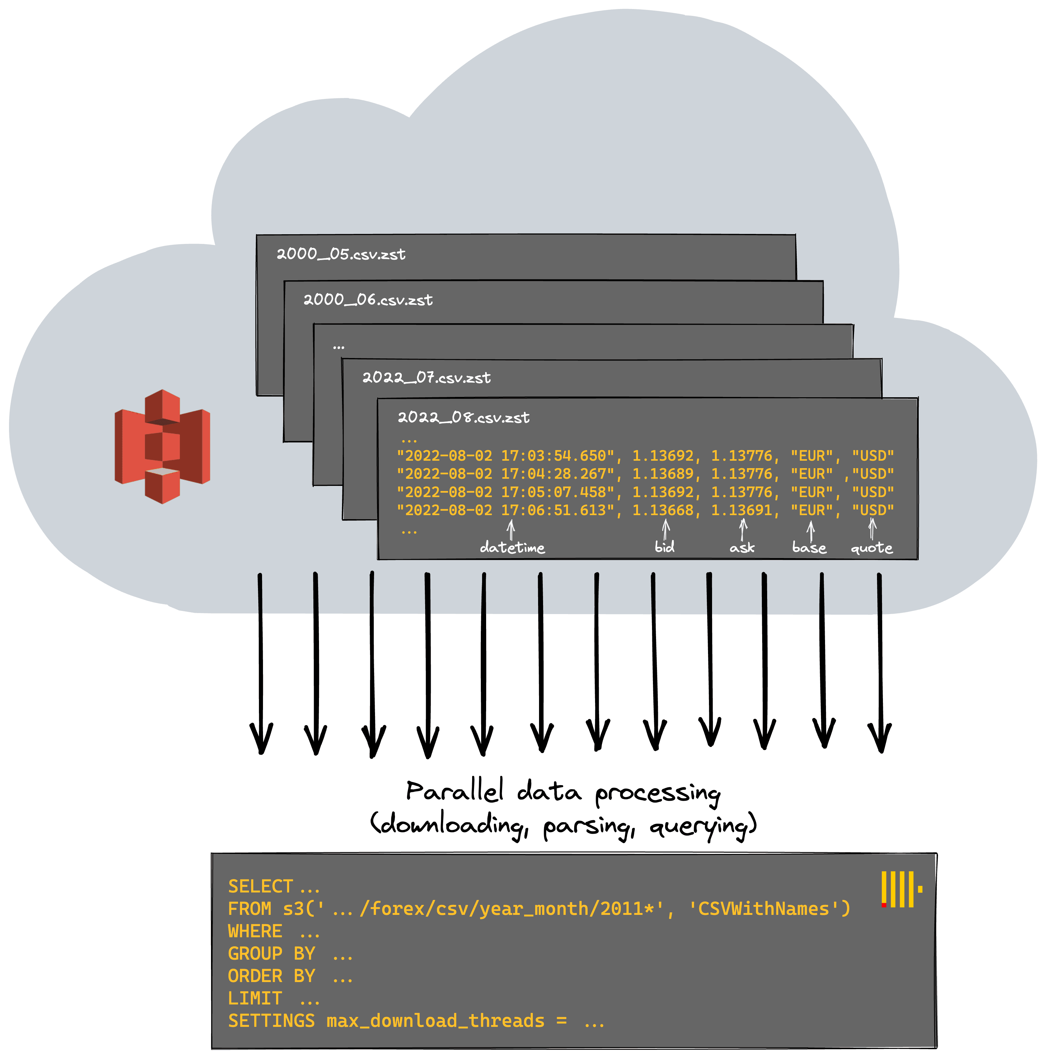
For optimal performance and in order to utilize all machine resources, ClickHouse attempts to parallelize as much work as possible, processing files in a streaming fashion. For S3, this means parallelizing both the downloading and parsing of files before the query is evaluated (again in parallel where possible) - interesting code comment here for more technical readers. By default, most steps will utilize the number of cores available.
Each of our ClickHouse Cloud nodes has eight cores. Via the setting max_download_threads, we increase the parallelization of the first stage and download more files in parallel - at the cost of greater memory consumption.
SELECT
    base,
    quote,
    avg(ask - bid) AS spread
FROM s3('https://datasets-documentation.s3.eu-west-3.amazonaws.com/forex/csv/year_month/*.csv.zst', 'CSVWithNames')
GROUP BY
    base,
    quote
ORDER BY spread ASC
LIMIT 10
SETTINGS max_download_threads = 12

// result omitted for brevity

10 rows in set. Elapsed: 435.508 sec. Processed 11.58 billion rows, 509.59 GB (26.59 million rows/s., 1.17 GB/s.)
Any further increases in threads are unlikely to equate to performance gains as we suffer from increased switching and poorer data access patterns. While this speeds up our query by about 33%, it's also not a magic bullet, and we are still restricted to the single node on which the query was received.
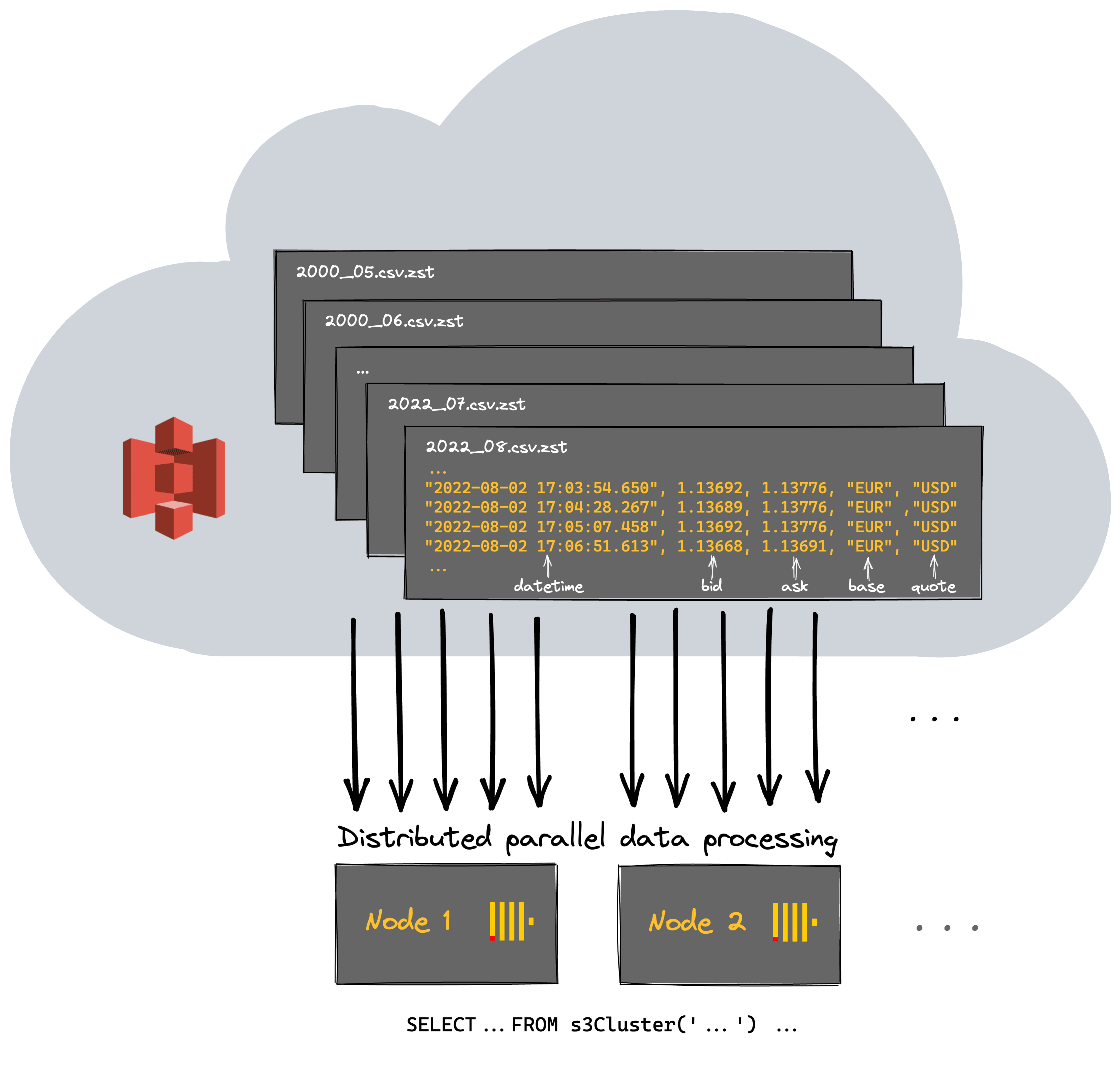
ClickHouse Cloud is a serverless offering with more than a single node responsible for computation. Ideally, we’d utilize all of our cluster resources for querying S3 and distribute the work across them. This can be achieved by simply using the s3Cluster function and specifying the cluster (default in the case of Cloud).
SELECT
    base,
    quote,
    avg(ask - bid) AS spread
FROM s3Cluster('default', 'https://datasets-documentation.s3.eu-west-3.amazonaws.com/forex/csv/year_month/*.csv.zst', 'CSVWithNames')
GROUP BY
    base,
    quote
ORDER BY spread ASC
LIMIT 10
SETTINGS max_download_threads = 12

// result omitted for brevity

10 rows in set. Elapsed: 226.449 sec. Processed 11.58 billion rows, 509.59 GB (51.14 million rows/s., 2.25 GB/s.)
A speedup of 2x suggests we have 2 nodes in our cluster, and at least initially linear scaling, confirmed with a simple query:
SELECT *
FROM system.clusters
FORMAT Vertical

Query id: 280a41fc-3d4d-4539-9947-31e41e2cc4cf

Row 1:
──────
cluster:                 default
shard_num:               1
shard_weight:            1
replica_num:             1
host_name:               c-orange-kq-53-server-0.c-orange-kq-53-server-headless.ns-orange-kq-53.svc.cluster.local
host_address:            10.21.142.214
port:                    9000
is_local:                0
user:
default_database:
errors_count:            0
slowdowns_count:         0
estimated_recovery_time: 0

Row 2:
──────
cluster:                 default
shard_num:               1
shard_weight:            1
replica_num:             2
host_name:               c-orange-kq-53-server-1.c-orange-kq-53-server-headless.ns-orange-kq-53.svc.cluster.local
host_address:            10.21.101.87
port:                    9000
is_local:                1
user:
default_database:
errors_count:            0
slowdowns_count:         0
estimated_recovery_time: 0

2 rows in set. Elapsed: 0.001 sec.
Optimizing this further is beyond the scope of this specific post and something for later, but by utilizing the full resources of the cluster, we’ve managed to query over 500GB at 50 million rows/sec.
Something a bit more interesting
Traders are always mindful of a widening spread when trading a currency pair. It represents the highest potential cost and can lead to the dreaded margin call when combined with leverage. Sudden changes in the spread that can spell disaster are usually associated with world events causing volatility and a lack of liquidity in the market. Below, we look for the biggest day changes in the spread for the EUR/USD pair using a window function. In this case, we use the parquet files for example purposes. Note that this isn’t always as performant as using csv files since parquet files can’t be parsed in parallel, reducing our throughput slightly.
SELECT
    base,
    quote,
    day,
    spread - any(spread) OVER (PARTITION BY base, quote ORDER BY base ASC, quote ASC, day ASC ROWS BETWEEN 1 PRECEDING AND CURRENT ROW) AS change
FROM
(
    SELECT
        base,
        quote,
        avg(ask - bid) AS spread,
        day
    FROM s3Cluster('default', 'https://datasets-documentation.s3.eu-west-3.amazonaws.com/forex/parquet/year_month/*.parquet')
    WHERE (base = 'EUR') AND (quote = 'USD')
    GROUP BY
        base,
        quote,
        toYYYYMMDD(datetime) AS day
    ORDER BY
        base ASC,
        quote ASC,
        day ASC
)
ORDER BY change DESC
LIMIT 5

┌─base─┬─quote─┬──────day─┬─────────────────change─┐
│ EUR  │ USD   │ 20010911 │  0.0008654604016672505 │
│ EUR  │ USD   │ 20201225 │ 0.00044359838480680655 │
│ EUR  │ USD   │ 20161225 │ 0.00022978220019175227 │
│ EUR  │ USD   │ 20081026 │ 0.00019250897043647882 │
│ EUR  │ USD   │ 20161009 │  0.0001777101378453994 │
└──────┴───────┴──────────┴────────────────────────┘

5 rows in set. Elapsed: 365.092 sec. Processed 11.58 billion rows, 613.82 GB (31.72 million rows/s., 1.68 GB/s.)
September 11th in 2001 understandably was pretty volatile, with it representing one of the most pivotal moments in modern history. Christmas might seem unusual, but markets typically become volatile in this period due to low volumes being traded, which causes the spread to widen. The 2008 datapoint is likely associated with the financial crisis.
If we assume the last ask price for a day is the close price for a currency pair (an approximation), we can see the biggest change for pairs of any currency pair. The argMax function allows us to obtain this price. Below we focus on the GBP since 2010 - using LIMIT BY to select one value per currency pair.
WITH daily_change AS
    (
        SELECT
            base,
            quote,
            day,
            close,
            close - any(close) OVER (PARTITION BY base, quote ORDER BY base ASC, quote ASC, day ASC ROWS BETWEEN 1 PRECEDING AND CURRENT ROW) AS change
        FROM
        (
            SELECT
                base,
                quote,
                day,
                argMax(ask, datetime) AS close
            FROM s3Cluster('default', 'https://datasets-documentation.s3.eu-west-3.amazonaws.com/forex/csv/year_month/20{1,2}*.csv.zst', 'CSVWithNames')
            WHERE (quote = 'GBP') OR (base = 'GBP')
            GROUP BY
                base,
                quote,
                toStartOfDay(datetime) AS day
            ORDER BY
                base ASC,
                quote ASC,
                day ASC
        )
        ORDER BY
            base ASC,
            quote ASC,
            day ASC
    )
SELECT base || '/' || quote as pair, day, round(close,3) as close, round(change,3) as change
FROM daily_change
WHERE day > '2016-01-02 00:00:00'
ORDER BY abs(change) DESC
LIMIT 1 BY
    base,
    quote
SETTINGS max_download_threads = 12

┌─pair────┬─────────────────day─┬────close─┬───change─┐
│ UKX/GBP │ 2020-03-15 00:00:00 │ 5218.507 │ -465.515 │
│ XAU/GBP │ 2016-06-23 00:00:00 │   994.92 │   139.81 │
│ GBP/JPY │ 2016-06-23 00:00:00 │  135.654 │  -19.225 │
│ GBP/NZD │ 2016-06-23 00:00:00 │     1.92 │   -0.141 │
│ GBP/CAD │ 2016-06-23 00:00:00 │    1.758 │   -0.138 │
│ GBP/USD │ 2016-06-23 00:00:00 │    1.345 │   -0.135 │
│ GBP/AUD │ 2016-06-23 00:00:00 │    1.833 │   -0.135 │
│ GBP/CHF │ 2016-06-23 00:00:00 │    1.312 │   -0.107 │
│ EUR/GBP │ 2016-06-23 00:00:00 │    0.817 │     0.05 │
└─────────┴─────────────────────┴──────────┴──────────┘

9 rows in set. Elapsed: 236.885 sec. Processed 10.88 billion rows, 478.74 GB (45.93 million rows/s., 2.02 GB/s.)
Unsurprisingly, the Brexit referendum was an exciting day to trade the GBP!
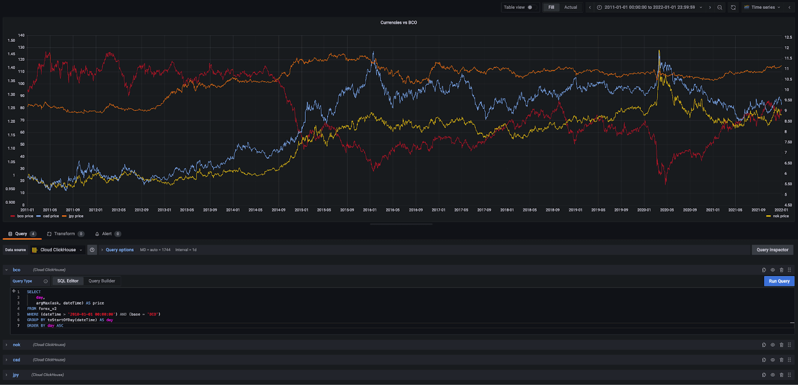
Our dataset also includes the BCO/USD pair tracking the Brent Crude Oil Price. Oil and currencies are inherently connected where a change in one can impact the other considerably. This correlation is more noticeable for USD currency pairs, where the pair currency is tied to an economy that depends heavily on crude exports. Currencies, such as Japanese Yen, which are associated with more diverse economies, typically have a looser correlation. We can confirm this hypothesis by using the correlation coefficient function in ClickHouse. The following query computes a correlation between the price of the NOK (Norwegian Krone), CAD (Canadian Dollar) and JPY (Japanese Yen) against the BCO price. These currencies represent the dependence of various economies on crude oil - Norway being the most dependant, Japan the least. Note our glob pattern means we only analyze files after 2011 - the earliest date available for BCO data.
SELECT
    corr(bco, cad),
    corr(bco, nok),
    corr(bco, jpy)
FROM
(
    SELECT
        day,
        anyIf(close, base = 'BCO') AS bco,
        anyIf(close, quote = 'CAD') AS cad,
        anyIf(close, quote = 'NOK') AS nok,
        anyIf(close, quote = 'JPY') AS jpy
    FROM
    (
        SELECT
            day,
            base,
            quote,
            argMax(ask, datetime) AS close
        FROM s3Cluster('default', 'https://datasets-documentation.s3.eu-west-3.amazonaws.com/forex/csv/year_month/20{1,2}{1,2}*.csv.zst', 'CSVWithNames')
        WHERE (datetime > '2011-01-01 00:00:00') AND (((base = 'USD') AND ((quote = 'CAD') OR (quote = 'NOK') OR (quote = 'JPY'))) OR (base = 'BCO'))
        GROUP BY
            toStartOfDay(datetime) AS day,
            quote,
            base
        ORDER BY
            day ASC,
            base ASC
    )
    GROUP BY day
    ORDER BY day ASC
)

┌─corr(bco, cad)─┬─corr(bco, nok)─┬─corr(bco, jpy)─┐
│    -0.82993394 │     -0.7567768 │    -0.55350846 │
└────────────────┴────────────────┴────────────────┘

1 row in set. Elapsed: 104.829 sec. Processed 3.39 billion rows, 149.33 GB (32.37 million rows/s., 1.42 GB/s.)
As expected, the NOK and CAD correlate tightly with the price of oil, whereas changes in BCO are less impactful on the JPY.
While we could continue querying the data in place, you may have noticed that the query times make any analysis quite time-consuming. A more real-time analysis requires us to insert the data into our ClickHouse nodes.
Using S3 as a source
The previous queries used ClickHouse’s S3 functions to query data in place. This offers flexibility and is useful for ad-hoc analysis. A common theme of all our S3 queries is the need to perform a linear scan over the entire dataset. We have no indexes or ability to optimize our queries besides organizing our files via naming and restricting with glob patterns.
At some point, users are prepared to pay an additional storage cost in exchange for significantly improved query performance (and likely productivity) by inserting the data into ClickHouse. Due to ClickHouse’s ability to compress data efficiently, the subsequent storage overhead is often a fraction of the original raw size.
To achieve this, we utilize the INSERT SELECT construct after first creating a table.
CREATE TABLE forex
(
    `datetime` DateTime64(3),
    `bid` Decimal(11, 5),
    `ask` Decimal(11, 5),
    `base` LowCardinality(String),
    `quote` LowCardinality(String)
)
ENGINE = MergeTree
ORDER BY (base, quote, datetime)

INSERT INTO forex
SELECT *
FROM s3Cluster('default', 'https://datasets-documentation.s3.eu-west-3.amazonaws.com/forex/csv/year_month/*.csv.zst', 'CSVWithNames')
SETTINGS max_download_threads = 12, max_insert_threads = 8
Note our primary key here is carefully selected for performance. The bid and ask price are represented as Decimal(11, 5), sufficient to represent our required precision. To accelerate this insert, we have used the setting max_insert_threads - increasing it to 8. Users should be cautious with this setting since it will increase memory overhead and may interfere with cluster background operations (merges). The s3Cluster function again allows us to distribute the work across the cluster. As of ClickHouse version 22.8, both the query and inserts will be fully distributed in this case. We can confirm the compression achieved by ClickHouse with a simple query. As shown, the original datasize has been significantly reduced.
SELECT table, formatReadableSize(sum(data_compressed_bytes)) AS compressed_size, formatReadableSize(sum(data_uncompressed_bytes)) AS uncompressed_size, sum(data_compressed_bytes) / sum(data_uncompressed_bytes) AS compression_ratio FROM system.columns WHERE (database = currentDatabase()) AND (table = 'forex') GROUP BY table ORDER BY table ASC ┌─table─┬─compressed_size─┬─uncompressed_size─┬──compression_ratio─┐ │ forex │ 102.97 GiB │ 280.52 GiB │ 0.36706997621862225│ └───────┴─────────────────┴───────────────────┴────────────────────┘✎
The true power of the above approach is the ability to be selective as to the data we insert. We can, in effect, slice and dice our data for faster analysis and only incur the storage costs for the subsets of interest. Our SELECT statement above could easily be modified to only insert data from the last 10 yrs where the USD is the base currency. Assume we have a table forex_usd of the identical schema shown above.
INSERT INTO forex_usd SELECT * FROM s3('https://datasets-documentation.s3.eu-west-3.amazonaws.com/forex/csv/year_month/2012*.csv.zst', 'CSVWithNames') WHERE (datetime > (now() - toIntervalYear(10))) AND (base = 'USD') Ok. 0 rows in set. Elapsed: 32.980 sec. Processed 598.28 million rows, 31.71 GB (18.14 million rows/s., 961.47 MB/s.) SELECT base, quote, min(datetime) FROM forex_usd GROUP BY base, quote Query id: c9f9b88b-dbb7-41f8-8cb9-3c22cf9ced8c ┌─base─┬─quote─┬───────────min(datetime)─┐ │ USD │ HUF │ 2012-09-09 17:01:19.220 │ │ USD │ NOK │ 2012-09-09 17:01:26.783 │ │ USD │ TRY │ 2012-09-09 17:01:17.157 │ │ USD │ DKK │ 2012-09-09 17:01:05.813 │ │ USD │ PLN │ 2012-09-09 17:01:12.000 │ │ USD │ MXN │ 2012-09-09 17:01:08.563 │ │ USD │ CZK │ 2012-09-09 17:01:23.000 │ │ USD │ SEK │ 2012-09-09 17:01:06.843 │ │ USD │ ZAR │ 2012-09-09 17:01:19.907 │ │ USD │ SGD │ 2012-09-09 17:01:03.063 │ │ USD │ JPY │ 2012-09-09 17:00:13.220 │ │ USD │ CAD │ 2012-09-09 17:00:15.627 │ │ USD │ HKD │ 2012-09-09 17:01:17.500 │ │ USD │ CHF │ 2012-09-09 17:00:17.347 │ └──────┴───────┴─────────────────────────┘✎
Real time analytics
Let’s repeat our earlier queries using a MergeTree table with the entire dataset loaded, to illustrate how the performance gains can be considerable:
First, let’s repeat the query that computed periods of high spread in the EUR/USD using our table instead of the s3 function.
SELECT base, quote, day, spread - any(spread) OVER (PARTITION BY base, quote ORDER BY base ASC, quote ASC, day ASC ROWS BETWEEN 1 PRECEDING AND CURRENT ROW) AS change FROM ( SELECT base, quote, avg(ask - bid) AS spread, day FROM forex WHERE (base = 'EUR') AND (quote = 'USD') GROUP BY base, quote, toYYYYMMDD(datetime) AS day ORDER BY base ASC, quote ASC, day ASC ) ORDER BY change DESC LIMIT 5 SETTINGS max_threads = 24 //results hidden for brevity 5 rows in set. Elapsed: 2.257 sec. Processed 246.77 million rows, 4.44 GB (109.31 million rows/s., 1.97 GB/s.)✎
3.5 seconds, 100x faster than 365! Note how our primary key avoids a full linear scan, reducing the number of processed rows.
What about our query assessing periods of high change in pairs involving the GBP?
WITH daily_change AS ( SELECT base, quote, day, close, close - any(close) OVER (PARTITION BY base, quote ORDER BY base ASC, quote ASC, day ASC ROWS BETWEEN 1 PRECEDING AND CURRENT ROW) AS change FROM ( SELECT base, quote, day, argMax(ask, datetime) AS close FROM forex WHERE (quote = 'GBP') OR (base = 'GBP') GROUP BY base, quote, toStartOfDay(datetime) AS day ORDER BY base ASC, quote ASC, day ASC ) ORDER BY base ASC, quote ASC, day ASC ) SELECT * FROM daily_change WHERE day > '2016-01-02 00:00:00' ORDER BY abs(change) DESC LIMIT 1 BY base, quote SETTINGS max_threads = 24 // results hidden for brevity 9 rows in set. Elapsed: 13.143 sec. Processed 2.12 billion rows, 29.71 GB (161.43 million rows/s., 2.26 GB/s.)✎
Our speedup, whilst less dramatic due to a looser constraint, is still 20x!
Generally, our performance gains will be determined by the effectiveness of our primary key and schema configuration. Optimizing keys and codes is a large topic beyond the scope of this post, but we encourage readers to explore starting with this guide. An astute reader will have noticed we also used the setting max_threads to increase the parallelization of our queries. Typically this is set to the number of cores, but increasing can improve the performance of some queries at the expense of higher memory. At somepoint CPU context switches will diminish higher gains and an optimal value is often query specific.
Time to visualize
Identifying trends and correlations often requires a visual representation. Performance in the seconds vs. minutes response times makes visual representations more viable. Fortunately, ClickHouse also integrates with a number of popular open-source tools. Below we’ll use Grafana to visualize the price of three currency pairs against the price of oil: CAD (Canadian Dollar), NOK (Norwegian Krone), and JPY (Japanese Yen).
All queries take the form:
SELECT day, argMax(ask, datetime) AS price FROM forex WHERE (datetime > '2010-01-01 00:00:00') AND (base = 'BCO') AND (quote = 'USD') GROUP BY toStartOfDay(datetime) AS day ORDER BY day ASC✎
Volatile market conditions in a currency pair are often seen as an excellent trading opportunity. In forex trading, this is computed as the standard deviation of the daily change in price, e.g., over the last 30 days. If the daily change is greater than this value, then we are entering a volatile period and a potential opportunity. We limit our analysis to the GBP/USD and plot this against the price.
SELECT day, stddevPop(change) OVER (PARTITION BY base, quote ORDER BY day ASC ROWS BETWEEN 30 PRECEDING AND CURRENT ROW) AS volatility, if(abs(change) > volatility, 'true', 'false') AS volatile FROM ( SELECT base, quote, day, close, close - any(close) OVER (PARTITION BY base, quote ORDER BY base ASC, quote ASC, day ASC ROWS BETWEEN 1 PRECEDING AND CURRENT ROW) AS change FROM ( SELECT base, quote, day, argMax(ask, datetime) AS close FROM forex WHERE (quote = 'USD') AND (base = 'GBP') AND (datetime > '2010-01-01 00:00:00') GROUP BY base, quote, toStartOfDay(datetime) AS day ORDER BY base ASC, quote ASC, day ASC ) ORDER BY base ASC, quote ASC, day ASC ) ORDER BY base ASC, quote ASC, day ASC SETTINGS max_threads = 24✎
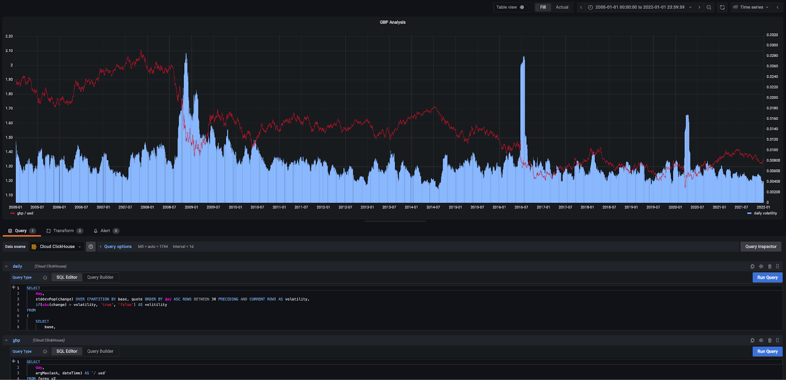
Clearly, the market was very volatile during the financial crash, Brexit, and the early days of the covid pandemic.
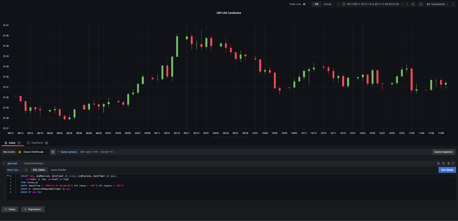
Candlestick charts are a common visualization technique in forex trading. These show the open, close, low, and high prices as bands with wicks. The color of the candlestick indicates the direction of the price. If the price of the candle closes above the opening price of the candle, then the price is moving upwards, and the candle will be green. If the candle is red, then the price has closed below the open. Fortunately, Grafana supports candlestick charts. Below we use a simple query to show the candlestick chart for the currency pair GBP/USD.
Bollinger Bands can provide a simple means of tracking trends for more detailed analysis at narrow points in time. These take a simple moving average (SMA) over the past 20 days and track a standard deviation away from that average on either side. These are, in turn, visualized as a simple moving average and an upper and lower band. When the distance between the bands widens, it illustrates increased market volatility for the currency in question. A smaller distance, by contrast, signals less volatility.
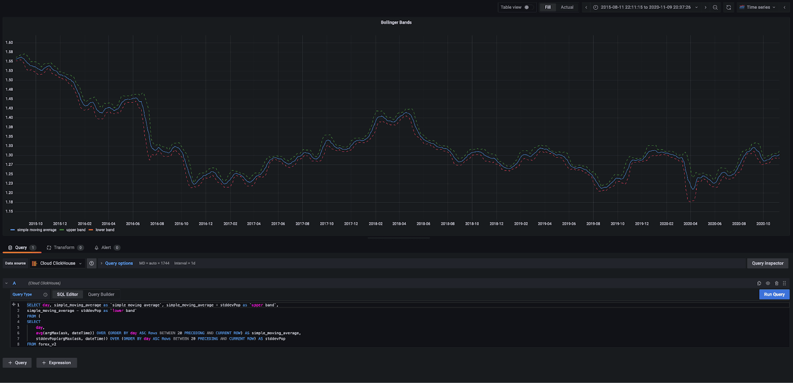
Traders use Bollinger bands intersecting with the candlesticks to determine buy and sell signals. For more detail, see here and here. Unfortunately, Grafana doesn’t allow these two visuals to be overlayed, but hopefully, they provide some inspiration.
Summary
In this blog post, we have explored querying forex data in S3 using ClickHouse for ad-hoc query demands, where users don’t need to access a dataset frequently, and therefore the cost of storing in ClickHouse is hard to justify. This approach is complemented by using S3 as a source of data for insertion into a table, where the full capabilities of ClickHouse can be exploited for real-time analytics. Finally, we have given readers a flavor of some of the visualization tools compatible with ClickHouse, which we will use more in future posts along with our forex dataset.