ClickHouse Release 24.2

Can you believe it’s already March?! Time is flying, but the good thing about another month going by is that we have another ClickHouse release for you to enjoy!

ClickHouse version 24.2 contains 18 new features 🎁 18 performance optimisations 🛷 49 bug fixes 🐛

As always, we send a special welcome to all the new contributors in 24.2! ClickHouse's popularity is, in large part, due to the efforts of the community that contributes. Seeing that community grow is always humbling.

Below are the names of the new contributors:

johnnymatthews, AlexeyGrezz, Aris Tritas, Charlie, Fille, HowePa, Joshua Hildred, Juan Madurga, Kirill Nikiforov, Nickolaj Jepsen, Nikolai Fedorovskikh, Pablo Musa, Ronald Bradford, YenchangChan, conicliu, jktng, mikhnenko, rogeryk, una, Кирилл Гарбар_

Hint: if you’re curious how we generate this list… here.

If you see your name here, please reach out to us...but we will be finding you on Twitter, etc as well.

You can also view the slides from the presentation.

Right, let's get into the features!

When processing files, ClickHouse will automatically detect the type of the file even if it doesn’t have a valid extension. For example, the following file foo contains data in JSON lines format:

$ cat foo

{"name": "John Doe", "age": 30, "city": "New York"}
{"name": "Jane Doe", "age": 25, "city": "Los Angeles"}
{"name": "Jim Beam", "age": 35, "city": "Chicago"}
{"name": "Jill Hill", "age": 28, "city": "Houston"}
{"name": "Jack Black", "age": 40, "city": "Philadelphia"}

Let’s try processing that file using the file function:

SELECT *
FROM file('foo')

┌─name───────┬─age─┬─city─────────┐
│ John Doe   │  30 │ New York     │
│ Jane Doe   │  25 │ Los Angeles  │
│ Jim Beam   │  35 │ Chicago      │
│ Jill Hill  │  28 │ Houston      │
│ Jack Black │  40 │ Philadelphia │
└────────────┴─────┴──────────────┘

5 rows in set. Elapsed: 0.003 sec.

Pretty cool. Let’s now write the content to say Parquet format:

SELECT *
FROM file('foo')
INTO OUTFILE 'bar'
FORMAT Parquet

And can we read that without telling ClickHouse the format?

SELECT *
FROM file('bar')

┌─name───────┬─age─┬─city─────────┐
│ John Doe   │  30 │ New York     │
│ Jane Doe   │  25 │ Los Angeles  │
│ Jim Beam   │  35 │ Chicago      │
│ Jill Hill  │  28 │ Houston      │
│ Jack Black │  40 │ Philadelphia │
└────────────┴─────┴──────────────┘

5 rows in set. Elapsed: 0.003 sec.

Of course, we can! The auto-detection also works when reading from URLs as well. So if we start up a local HTTP server around the above files:

python -m http.server

We can then read them like this:

SELECT *
FROM url('http://localhost:8000/bar')

┌─name───────┬─age─┬─city─────────┐
│ John Doe   │  30 │ New York     │
│ Jane Doe   │  25 │ Los Angeles  │
│ Jim Beam   │  35 │ Chicago      │
│ Jill Hill  │  28 │ Houston      │
│ Jack Black │  40 │ Philadelphia │
└────────────┴─────┴──────────────┘

That’s enough examples for now, but you can also use this functionality with the s3, hdfs, and azureBlobStorage table functions.

If you've ever had to quickly interpret a large number in a query result, this feature is for you. When you return a single numerical column, if the value in that column is bigger than 1 million, the readable quantity will be displayed as a comment alongside the value itself.

SELECT 765432198

┌─765432198─┐
│ 765432198 │ -- 765.43 million
└───────────┘

Before this release if you defined a view on a table, for a user to access the view they also needed to have access to the table. This wasn’t ideal and in 24.2 we’ve added the SQL SECURITY and DEFINER specifications for CREATE VIEW queries to solve this problem.

Let’s say that we have a payroll table for our company that contains employees’ names, departments, salaries, and address details. We might want to make it possible for the HR team to access all the information but also allow other users to see employee names and departments.

Let’s first create a table and populate it:

CREATE TABLE payroll (
  name String,
  address String,
  department LowCardinality(String),
  salary UInt32
)
Engine = MergeTree
ORDER BY name;

INSERT INTO payroll (`name`, `address`, `department`, `salary`) VALUES
('John Doe', '123 Maple Street, Anytown, AT 12345', 'HR', 50000),
('Jane Smith', '456 Oak Road, Sometown, ST 67890', 'Marketing', 55000),
('Emily Jones', '789 Pine Lane, Thistown, TT 11223', 'IT', 60000),
('Michael Brown', '321 Birch Blvd, Othertown, OT 44556', 'Sales', 52000),
('Sarah Davis', '654 Cedar Ave, Newcity, NC 77889', 'HR', 53000),
('Daniel Wilson', '987 Elm St, Oldtown, OT 99000', 'IT', 62000),
('Laura Martinez', '123 Spruce Way, Mytown, MT 22334', 'Marketing', 56000),
('James Garcia', '456 Fir Court, Yourtown, YT 33445', 'Sales', 51000);

We have a couple of users - Alice who’s in the HR team and Bob who’s in the engineering team. Alice is in the HR team and has access to the payroll table, Bob does not!

CREATE USER alice IDENTIFIED WITH sha256_password BY 'alice';
GRANT SELECT ON default.payroll TO alice;
GRANT SELECT ON default.employees TO alice  WITH GRANT OPTION;

CREATE USER bob IDENTIFIED WITH sha256_password BY 'bob';

Alice creates a view called employees:

CREATE VIEW employees	
DEFINER = alice SQL SECURITY DEFINER
AS 
SELECT name, department
FROM payroll;

And then Alice gives access to that view to herself and Bob:

GRANT SELECT ON default.employees TO alice;
GRANT SELECT ON default.employees TO bob;

If we then log in as Bob:

clickhouse client -u bob

We can query the employees table:

SELECT *
FROM employees

┌─name───────────┬─department─┐
│ Daniel Wilson  │ IT         │
│ Emily Jones    │ IT         │
│ James Garcia   │ Sales      │
│ Jane Smith     │ Marketing  │
│ John Doe       │ HR         │
│ Laura Martinez │ Marketing  │
│ Michael Brown  │ Sales      │
│ Sarah Davis    │ HR         │
└────────────────┴────────────┘

But he can’t query the underlying payroll table, which is what we’d expect:

SELECT *
FROM payroll

Received exception from server (version 24.3.1):
Code: 497. DB::Exception: Received from localhost:9000. DB::Exception: bob: Not enough privileges. To execute this query, it's necessary to have the grant SELECT(name, address, department, salary) ON default.payroll. (ACCESS_DENIED)

In recent blog posts, we have explored how ClickHouse can be used as a vector database when users need highly performant linear scans for accurate results and/or the ability to combine vector search with filtering and aggregating on metadata through SQL. Users can use these capabilities to provide context to LLM-based applications through Retrieval-augmented generation (RAG) pipelines. Our investment in the underlying support for Vector search continues with efforts recently focused on improving the performance of linear scans - specifically the family of distance functions that calculate the distance between 2 vectors. For background, we recommend this post and a recent video from our very own Mark:

While query performance for vector search can easily be I/O bound for larger datasets, many users simply need to search smaller datasets with SQL that fit into memory. In these cases, performance in ClickHouse can become CPU-bound. Efforts to ensure this code is properly vectorized and uses the latest instruction sets can therefore provide significant improvement and move performance to being limited by memory bandwidth - for machines with DDR-5 this can mean even higher scan performance.

In 24.2, we’re pleased to announce that the cosineDistance, dotProduct, and L2Distance (euclidean distance) functions have all been optimized to exploit the latest instruction sets. In the case of x86, this means the use of the fused multiply-add (FMA) and horizontal add-reduce operations with AVX-512 instructions and auto-vectorization for ARM.

As an example of the potential improvements, consider the following glove dataset popularized in the almost official ANN benchmarks. This particular subset, which we’ve made available in Parquet (2.5GiB), consists of 2.1m vectors trained from 840B CommonCrawl tokens. Each vector in this set has 300 dimensions and represents a word. Given the simple schema, this takes a few seconds to load into ClickHouse:

CREATE TABLE glove
(
  `word` String,
  `vector` Array(Float32)
)
ENGINE = MergeTree
ORDER BY word;

INSERT INTO glove SELECT *
FROM s3('https://datasets-documentation.s3.eu-west-3.amazonaws.com/glove/glove_840b_300d.parquet')

0 rows in set. Elapsed: 49.779 sec. Processed 2.20 million rows, 2.66 GB (44.12 thousand rows/s., 53.44 MB/s.)
Peak memory usage: 1.03 GiB.

Machine specification: i3en.3xlarge - 12vCPU Intel(R) Xeon(R) Platinum 8259CL CPU @ 2.50GHz, 96GiB RAM

We can compare performance between versions of ClickHouse by finding those words closest to the vector for a specific word. For example, in 23.12:

WITH 'dog' AS search_term,
(
  SELECT vector
  FROM glove
  WHERE word = search_term
  LIMIT 1
) AS target_vector
SELECT word, cosineDistance(vector, target_vector) AS score
FROM glove
WHERE lower(word) != lower(search_term)
ORDER BY score ASC
LIMIT 5

┌─word────┬──────score─┐
│ dogs    │ 0.11640692 │
│ puppy   │ 0.14147866 │
│ pet     │ 0.19425482 │
│ cat     │ 0.19831467 │
│ puppies │ 0.24826884 │
└─────────┴────────────┘

5 rows in set. Elapsed: 0.407 sec. Processed 2.14 million rows, 2.60 GB (5.25 million rows/s., 6.38 GB/s.)
Peak memory usage: 248.94 MiB.

What's important here is that this dataset fits into the FS cache, as shown by its compressed size on disk:

SELECT
	name,
	formatReadableSize(sum(data_compressed_bytes)) AS compressed_size,
	formatReadableSize(sum(data_uncompressed_bytes)) AS uncompressed_size,
	round(sum(data_uncompressed_bytes) / sum(data_compressed_bytes), 2) AS ratio
FROM system.columns
WHERE table LIKE 'glove'
GROUP BY name
ORDER BY name DESC

┌─name───┬─compressed_size─┬─uncompressed_size─┬─ratio─┐
│ word   │ 13.41 MiB       │ 18.82 MiB         │   1.4 │
│ vector │ 2.46 GiB        │ 2.47 GiB          │     1 │
└────────┴─────────────────┴───────────────────┴───────┘

2 rows in set. Elapsed: 0.003 sec.

The total size of the word and vector columns is around 2.65 GB, which comfortably fits into memory.

In 24.2, the same query improves by over 25%:

5 rows in set. Elapsed: 0.286 sec. Processed 1.91 million rows, 2.32 GB (6.68 million rows/s., 8.12 GB/s.)
Peak memory usage: 216.89 MiB.

These differences will vary by processor, dataset size, vector cardinality, and RAM performance.

Before 24.2, the dotProduct function was not vectorized. While ensuring this was as efficient as possible we noticed that the function also performed the necessary unpacking of any const arguments (the most common use case i.e. we pass a constant vector for comparison) which led to unnecessary memory copies. This meant the actual function runtime was dominated by memory operations - vectorization in this case was a comparatively small gain. Once eliminated performance was improved a staggering 270x on automated benchmarks!

While it's not worth comparing performance to previous versions for this function (they are a little embarrassing :)), we thought we’d use the opportunity to note that the improvements allow us to demonstrate a nice performance optimization users can now exploit.

Readers may recall that the cosine distance and dot product are closely related. More specifically, cosine distance measures the cosine of the angle between two vectors in a multi-dimensional space. It is derived from the cosine similarity, with cosine distance defined as 1 - cosine similarity. The cosine similarity is calculated as the dot product of the vectors divided by the product of their magnitudes i.e. 1- ((a.b)/||a||||b||). Conversely, the dot product measures the sum of the products of the corresponding entries of the two sequences of numbers i.e. vectors A and B with components ai and bi, the dot product is A⋅B=∑ai​bi​.

Cosine distance and dot product become particularly related when you normalize the vectors (i.e., when the magnitude of both vectors is 1). In this case, the cosine similarity is exactly the dot product because the denominators in the cosine similarity formula (the magnitudes of the vectors) are both 1, thus canceling out. Our cosine distance thus simply becomes 1-(a.b).

How can we exploit this?

We can normalize our vectors at insert time using the L2Norm function (vector magnitude) allowing us to use the dotProduct function at query time. The main motivation for this is that the dotProduct function is computationally simpler (we don’t have to compute the magnitude for each vector), thus potentially saving us a little query time.

To perform normalization at query time:

INSERT INTO glove
SETTINGS schema_inference_make_columns_nullable = 0
SELECT
	word,
	vector / L2Norm(vector) AS vector
FROM s3('https://datasets-documentation.s3.eu-west-3.amazonaws.com/glove/glove_840b_300d.parquet')
SETTINGS schema_inference_make_columns_nullable = 0

0 rows in set. Elapsed: 51.699 sec. Processed 2.20 million rows, 2.66 GB (42.48 thousand rows/s., 51.46 MB/s.)

Our query from earlier thus becomes:

WITH
	'dog' AS search_term,
	(
    	SELECT vector
    	FROM glove
    	WHERE word = search_term
    	LIMIT 1
	) AS target_vector
SELECT
	word,
	1 - dotProduct(vector, target_vector) AS score
FROM glove
WHERE lower(word) != lower(search_term)
ORDER BY score ASC
LIMIT 5

┌─────────┬─────────────────────┐
│ word    │ score               │
├─────────┼─────────────────────┤
│ dogs    │ 0.11640697717666626 │
│ puppy   │ 0.1414787769317627  │
│ pet     │ 0.19425475597381592 │
│ cat     │ 0.19831448793411255 │
│ puppies │ 0.24826878309249878 │
└─────────┴─────────────────────┘


5 rows in set. Elapsed: 0.262 sec. Processed 1.99 million rows, 2.42 GB (7.61 million rows/s., 9.25 GB/s.)
Peak memory usage: 226.29 MiB.

This query takes 0.262 seconds compared to 0.286 seconds when using cosine similarity - a small time saving when compared to our original query, but every ms counts!

There is a PR still pending that will fix both correctness and performance of the dotProduct function, which should be merged soon.

With traditional insert queries, data is inserted into a table synchronously: When the query gets received by ClickHouse, the data is immediately written to the database storage in the form of a data part. For optimal performance, data needs to be batched, and generally, we should avoid creating too many small inserts too frequently.

Asynchronous inserts shift data batching from the client side to the server side: data from insert queries is inserted into a buffer first and then written to the database storage later or asynchronously respectively. This is handy, especially for scenarios where many concurrent clients insert data frequently into a table, the data should be analyzed in real-time, and delays caused by client-side batching are unacceptable. For example, observability use cases frequently involve thousands of monitoring agents continuously sending small amounts of event and metrics data. Such scenarios can utilize the asynchronous insert mode, illustrated by the following diagram:

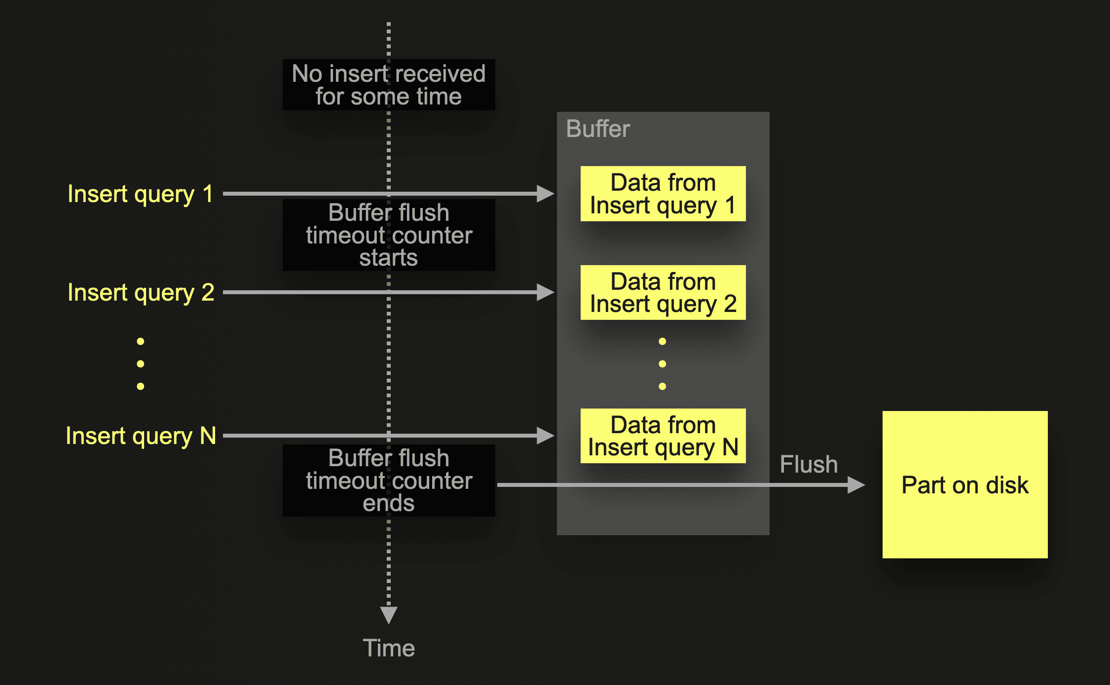
In the example scenario in the diagram above, ClickHouse receives an asynchronous insert query 1 for a specific table after a period of no insert activity for this table. After receiving insert query 1, the query’s data is inserted into an in-memory buffer, and the default buffer flush timeout counter starts. Before the counter ends, and therefore the buffer gets flushed, the data of other asynchronous insert queries from the same or other clients can be collected in the buffer. Flushing the buffer will create a data part on disk containing the combined data from all insert queries received before the flush.

Note that with the default return behavior, all insert queries only return with an acknowledgment of the insert to the sender after the buffer flush occurs. In other words, the client-side call sending the insert query is blocked until the next buffer flush occurs. As a consequence, infrequent inserts have a higher latency. We sketch this below:

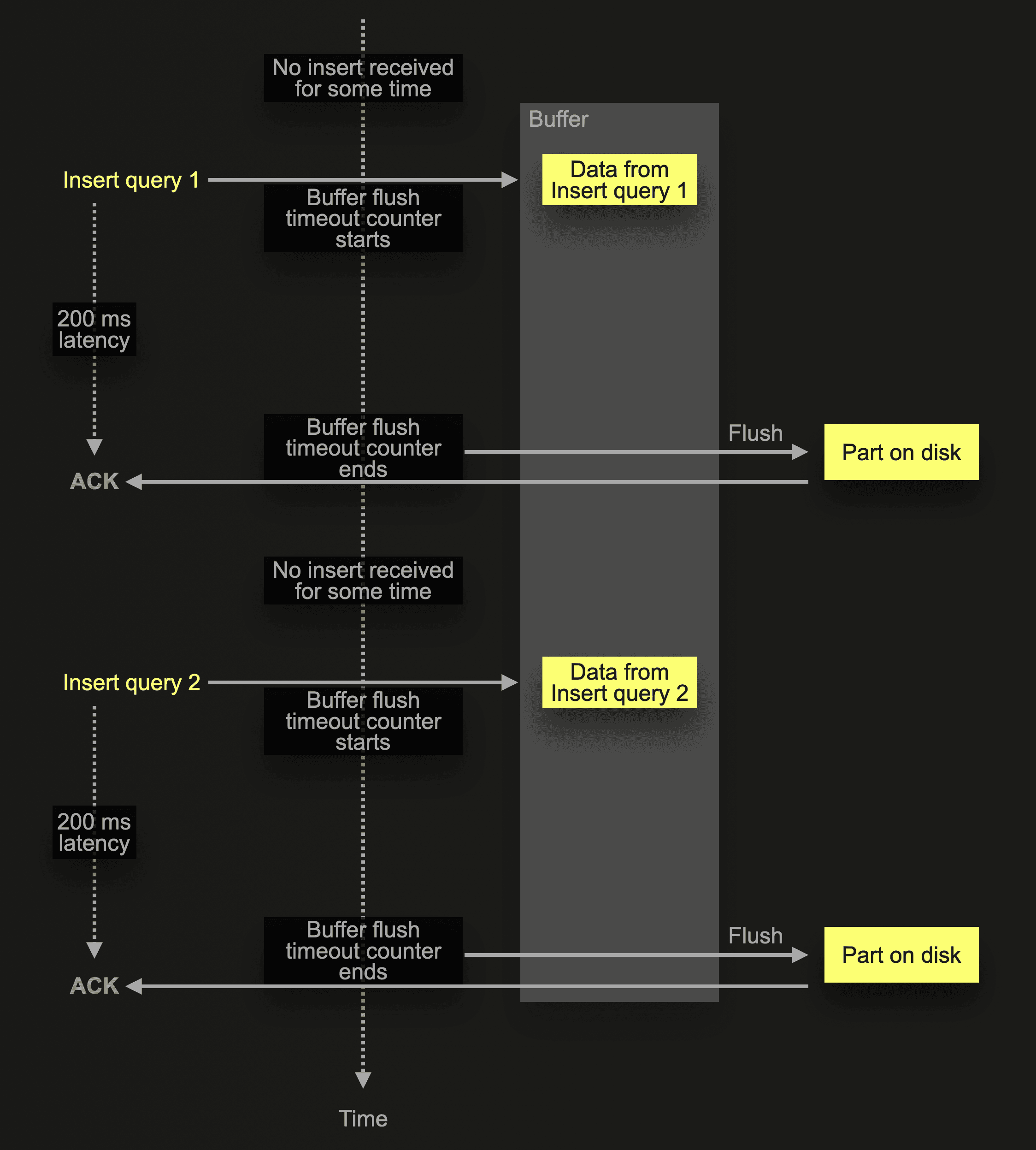
The extreme case scenario above shows infrequent insert queries. ClickHouse receives an asynchronous insert query 1 after a period of no insert activity for a table. This triggers a new buffer flush cycle with the default buffer flush timeout, meaning that the sender of that query needs to wait for the complete default buffer flush time (200 ms for OSS or 1000 ms for ClickHouse Cloud) before receiving an acknowledgment of the insert. Similarly, the sender of insert query 2 experiences a high insert latency.

The adaptive asynchronous insert buffer flush timeout introduced in ClickHouse 24.2 solves this problem by using an adaptive algorithm for automatically adjusting the buffer flush timeout based on the frequency of inserts:

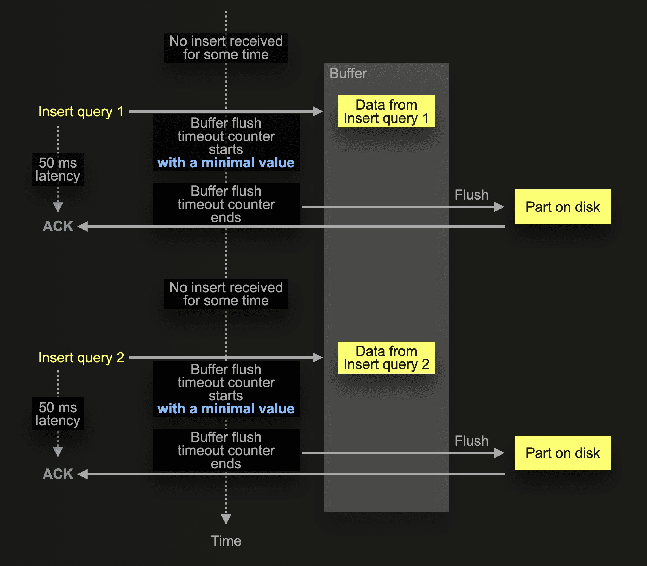
For the extreme case scenario shown before with some infrequent insert queries, the buffer flush timeout counter now starts with a minimal value (50 ms). Therefore the data from these queries is written to disk much sooner. It is ok to almost immediately write small data amounts to disk, as the frequency is low. Therefore there is no risk of the Too many parts safeguard kicking in.

Frequent inserts work as before. They will be delayed and combined:

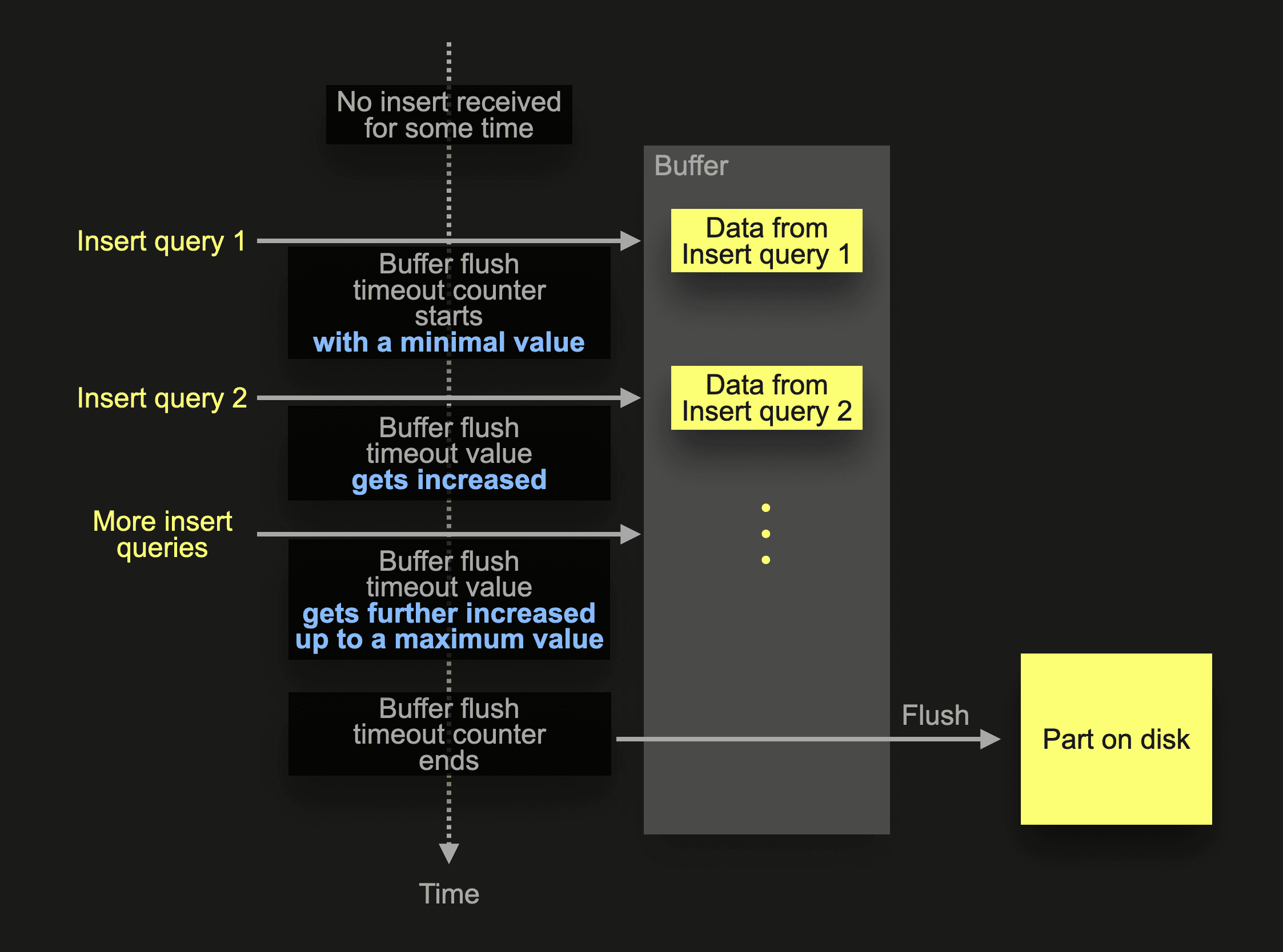
When ClickHouse receives insert query 1 after a period of no insert activity for a table, the buffer flush timeout counter starts with a minimal value, which is automatically adjusted up to a maximum value when additional inserts occur frequently (and gets also adjusted back down when the insert frequency decreases).

In summary, frequent inserts work as before. They will be delayed and combined together. Infrequent inserts, however, will not be delayed much and behave like synchronous inserts. \ You can just enable async insert and stop worrying. 😀

Let’s demonstrate this with an example. For this, we start a ClickHouse 24.2 instance and create a simplified version of the table from our UpClick observability example application:

CREATE TABLE default.upclick_metrics (
    `url` String,
    `status_code` UInt8,
    `city_name_en` String
) ENGINE = MergeTree
ORDER BY (url, status_code, city_name_en);

Now we can use this simple Python script (using the ClickHouse Connect Python driver) to send 10 small asynchronous inserts to our ClickHouse instance. Note that we explicitly enable the default return behavior by setting wait_for_async_insert to 1, and we increase the buffer flush timeout to 2 seconds (to demonstrate adaptive async inserts better).

import clickhouse_connect
import time

client = clickhouse_connect.get_client(...)

for _ in range(10):
    start_time = time.time()
    client.insert(
        database='default',
        table='upclick_metrics',
        data=[['clickhouse.com', 200, 'Amsterdam']],
        column_names=['url', 'status_code', 'city_name_en'],
        settings={
            'async_insert':1,
            'wait_for_async_insert':1,
            'async_insert_busy_timeout_ms':2000,
            'async_insert_use_adaptive_busy_timeout':0}
    )
    end_time = time.time()
    print(str(round(end - start, 2)) + ' seconds')
    time.sleep(1)

The script measures and prints the insert’s latency (in seconds) for each insert and then sleeps for one second to simulate infrequent inserts.

We run the script with disabled adaptive asynchronous insert buffer flush timeout (async_insert_use_adaptive_busy_timeout is set to 0), and the output is:

2.03 seconds
2.02 seconds
2.03 seconds
2.02 seconds
2.04 seconds
2.02 seconds
2.03 seconds
2.03 seconds
2.03 seconds
2.03 seconds

We can see the high latency of 2 seconds for the infrequent inserts.

However, when we run the script with enabled adaptive asynchronous insert buffer flush timeout (async_insert_use_adaptive_busy_timeout is set to 1) and all other settings identical to the run above, the output is:

0.07 seconds
0.06 seconds
0.08 seconds
0.08 seconds
0.07 seconds
0.07 seconds
0.07 seconds
0.08 seconds
0.07 seconds
0.08 seconds

The latency for the infrequent inserts is drastically reduced.

We don’t precisely see the minimal buffer flush timeout of 50 ms here because of additional latencies overhead from the Python driver mechanics, serverside query parsing, and time for sending the query to ClickHouse, etc.