We are super excited to share a trove of amazing features in 23.10
And, we already have a date for the 23.11 release, please register now to join the community call on December 5th at 9:00 AM (PDT) / 6:00 PM (CET).
Release Summary
23 new features. 26 performance optimisations. 60 bug fixes.
A small subset of highlighted features are below…But the release covers new SHOW MERGES and SHOW SETTINGS commands, new byteSwap, arrayRandomSample, jsonMergePatch, formatQuery, formatQuerySingleLine functions, argMin and argMax as combinators, parameterized ALTER command with partitions, untuple function with better names, enforcing projections, allowing tables without a primary key, and so…much…more.
New Contributors
As always, we send a special welcome to all the new contributors in 23.10! ClickHouse's popularity is, in large part, due to the efforts of the community that contributes. Seeing that community grow is always humbling.
If you see your name here, please reach out to us...but we will be finding you on twitter, etc as well.
AN, Aleksa Cukovic, Alexander Nikolaev, Avery Fischer, Daniel Byta, Dorota Szeremeta, Ethan Shea, FFish, Gabriel Archer, Itay Israelov, Jens Hoevenaars, Jihyuk Bok, Joey Wang, Johnny, Joris Clement, Lirikl, Max K, Priyansh Agrawal, Sinan, Srikanth Chekuri, Stas Morozov, Vlad Seliverstov, bhavuk2002, guoxiaolong, huzhicheng, monchickey, pdy, wxybear, yokofly
Largest Triangle Three Buckets
Contributed by Sinan
Largest Triangle Three Buckets is an algorithm for downsampling data to make it easier to visualize. It tries to retain the visual similarity of the initial data while reducing the number of points. In particular, it seems to be very good at retaining local minima and maxima, which are often lost with other downsampling methods.
We’re going to see how it works with help from the Kaggle SF Bay Area Bike Share dataset, which contains one CSV file that tracks the number of docks available per station on a minute-by-minute basis.
Let’s create a database:
CREATE DATABASE BikeShare;
USE BikeShare;
And then create a table, status, populated by the status.csv file:
create table status engine MergeTree order by (station_id, time) AS
from file('Bay Area Bikes.zip :: status.csv', CSVWithNames)
SELECT *
SETTINGS schema_inference_make_columns_nullable=0;

SELECT formatReadableQuantity(count(*))
FROM status

┌─formatReadableQuantity(count())─┐
│ 71.98 million                   │
└─────────────────────────────────┘
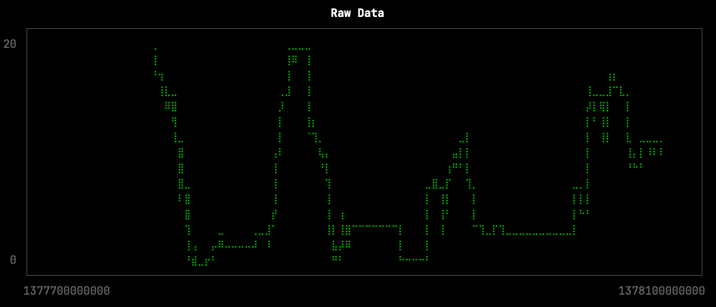
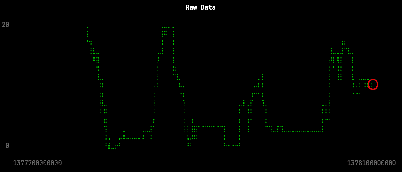
Raw data
Let’s first have a look at the raw data for one of the stations over a period of a few days. There are 4,537 points returned by the following query, which is stored in the file raw.sql:
from BikeShare.status select toUnixTimestamp64Milli(time), docks_available
where toDate(time) >= '2013-08-29' and toDate(time) <= '2013-09-01'
and station_id = 70
FORMAT CSV
We can visualize the docks available over time by running the following query:
clickhouse local --path bikeshare.chdb < raw.sql |
uplot line -d, -w 100 -t "Raw Data"
Next, we’re going to see what happens if we reduce the number of points by roughly 10x, which we can do by averaging the points in buckets of 10 minutes. This query will be stored in the file avg.sql and is shown below:
WITH buckets AS (
  SELECT
    toStartOfInterval(time, INTERVAL 10 minute) AS bucket,
    AVG(docks_available) AS average_docks_available,
    AVG(toUnixTimestamp64Milli(time)) AS average_bucket_time
  FROM BikeShare.status
  where toDate(time) >= '2013-08-29' and toDate(time) <= '2013-09-01'
  AND (station_id = 70)
  GROUP BY bucket
  ORDER BY bucket
)
SELECT average_bucket_time, average_docks_available
FROM buckets
FORMAT CSV
We can generate the visualization like this:
clickhouse local --path bikeshare.chdb < avg.sql |
uplot line -d, -w 100 -t "Average every 5 mins"
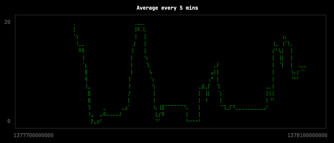
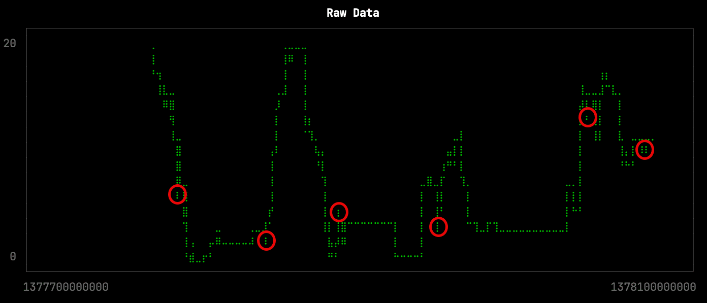
This downsampling isn’t too bad, but it has lost some of the more subtle changes in the shape of the curve. The missing changes are circled in red on the raw data visualization:
Let’s see how the Largest Triangle Three Buckets algorithm does. The query (lttb.sql) is shown below:
from BikeShare.status
select untuple(arrayJoin(
  largestTriangleThreeBuckets(50)(
    toUnixTimestamp64Milli(time), docks_available
)))
where toDate(time) >= '2013-08-29' and toDate(time) <= '2013-09-01' AND station_id = 70
FORMAT CSV
And we can generate the visualization like this:
clickhouse local --path bikeshare.chdb < lttb.sql |
uplot line -d, -w 100 -t "Largest Triangle Three Buckets"
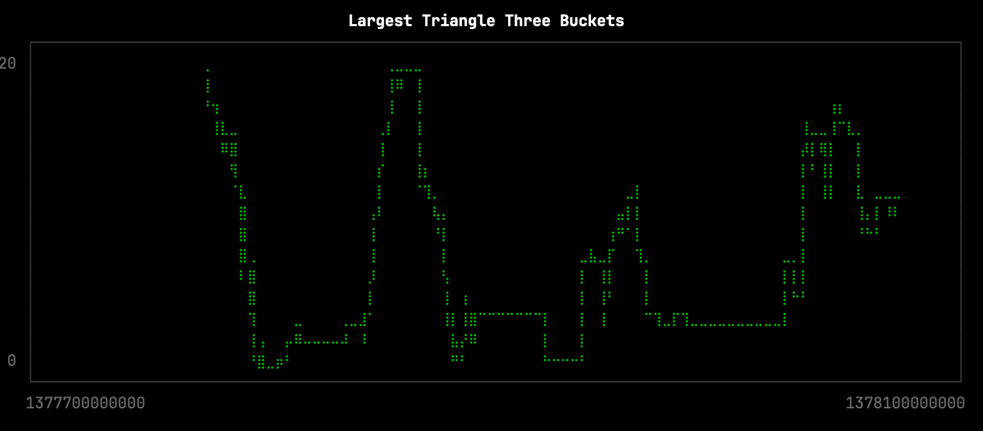
From a visual inspection, this version of the visualization is only missing the following local minima:
arrayFold
Contributed by Lirikl
ClickHouse provides SQL with many extensions and powerful improvements that make it more friendly for analytical tasks. One example of this ClickHouse superset of SQL is extensive support for arrays. Arrays are well-known to users of other programming languages like Python and JavaScript. They are generally useful for modeling and solving a wide range of problems in an elegant and simple way. ClickHouse has over 70 functions for processing arrays, with many of these functions being higher-order functions providing a high level of abstraction, allowing you to express complex operations on arrays in a concise and declarative manner. We proudly announce that this family of array functions now has a new, long-awaited, and most powerful member: arrayFold.
arrayFold is equivalent to the Array.reduce function in JavaScript and is used to fold or reduce the elements in an array from left to right by applying a lambda-function to the array elements in a cumulative manner, starting from the leftmost element and accumulating a result as it processes each element. This cumulative process can be thought of as folding the elements of the array together.
The following is a simple example where we use arrayFold for calculating the sum of all elements of the array [10, 20, 30]:
SELECT arrayFold((acc, v) -> (acc + v), [10, 20, 30],  0::UInt64) AS sum

┌─sum─┐
│  60 │
└─────┘
Note that we are passing both a lambda function (acc, v) -> (acc + v) and an initial accumulator value 0 in the example call of arrayFold above.
The lambda function is then called with acc set to the initial accumulator value 0 and v set to the first (most left) array element 10. Next, the lambda function is called with acc set to the result of the previous step and v set to the second array element 20. This process continues, iteratively folding the array elements from left to right until the end of the array is reached, producing a final result, 60.
This diagram visualizes how the + operator from the body of our lambda function is cumulatively applied to the initial accumulator and all array elements from left to right:

We used the example above just as an introduction. We could have used arraySum or arrayReduce(sum) for calculating the sum of all array elements. But arrayFold is far more capable. It is one of the most generic and flexible members of the ClickHouse array function family that can be used to perform a wide range of operations on arrays, such as aggregating, filtering, mapping, grouping, and more complex tasks.
The possibility to (1) provide a custom folding function in the form of a lambda function, and to (2) hold, inspect, and shape the folding state (accumulator) on each iteration step is a powerful combination allowing complex data processing in a concise and composable way. We demonstrate this with a more complex example. Almost exactly a year ago, we challenged our community to formulate a query reconstructing the git blame command, offering a t-shirt to the first solution. We even mentioned:
“Reconstructing this from a history of commits is particularly challenging - especially since ClickHouse doesn’t currently have an arrayFold function which iterates with the current state.”
Well, now is your chance to win the t-shirt 🤗
The following is a related and simplified example modeling a ClickHouse-powered text editor providing unlimited time/version travel where we only store the per-line changes and utilize arrayFold for easily reconstructing the complete text for each version (or point in time).
We create the table for storing the line change history (per version, we could also use a DateTime field to track the times of changes):
CREATE OR REPLACE TABLE line_changes
(
    version UInt32,
    line_change_type Enum('Add' = 1, 'Delete' = 2, 'Modify' = 3),
    line_number UInt32,
    line_content String
)
ENGINE = MergeTree
ORDER BY time;
We store a history of line changes:
INSERT INTO default.line_changes VALUES
(1, 'Add'   , 1, 'ClickHouse provides SQL'),
(2, 'Add'   , 2, 'with improvements'),
(3, 'Add'   , 3, 'that makes it more friendly for analytical tasks.'),
(4, 'Add'   , 2, 'with many extensions'),
(5, 'Modify', 3, 'and powerful improvements'),
(6, 'Delete', 1, ''),
(7, 'Add'   , 1, 'ClickHouse provides a superset of SQL');
We create three user-defined functions for manipulation array content (we create these UDFs just for readability; alternatively, we could have inlined their body into the main query below):
-- add a string (str) into an array (arr) at a specific position (pos)
CREATE OR REPLACE FUNCTION add AS (arr, pos, str) ->
  arrayConcat(arraySlice(arr, 1, pos-1), [str], arraySlice(arr, pos));

-- delete the element at a specific position (pos) from an array (arr)
CREATE OR REPLACE FUNCTION delete AS (arr, pos) ->
  arrayConcat(arraySlice(arr, 1, pos-1), arraySlice(arr, pos+1));

-- replace the element at a specific position (pos) in an array (arr)
CREATE OR REPLACE FUNCTION modify AS (arr, pos, str) ->
  arrayConcat(arraySlice(arr, 1, pos-1), [str], arraySlice(arr, pos+1));
We create a parameterized view with the main query utilizing arrayFold:
CREATE OR REPLACE VIEW text_version AS
WITH T1 AS (
  SELECT arrayZip(
    groupArray(line_change_type),
    groupArray(line_number),
    groupArray(line_content)) as line_ops
  FROM (SELECT * FROM line_changes
        WHERE version <= {version:UInt32} ORDER BY version ASC)
)
SELECT arrayJoin(
  arrayFold((acc, v) ->
    if(v.'change_type' = 'Add',       add(acc, v.'line_nr', v.'content'),
    if(v.'change_type' = 'Delete', delete(acc, v.'line_nr'),
    if(v.'change_type' = 'Modify', modify(acc, v.'line_nr', v.'content'), []))),
    line_ops::Array(Tuple(change_type String, line_nr UInt32, content String)),
    []::Array(String))) as lines
FROM T1;
We travel through text versions:
SELECT * FROM text_version(version = 2);

┌─lines─────────────────────────────────────────────┐
│ ClickHouse provides SQL                           │
│ that makes it more friendly for analytical tasks. │
└───────────────────────────────────────────────────┘


SELECT * FROM text_version(version = 3);

┌─lines─────────────────────────────────────────────┐
│ ClickHouse provides SQL                           │
│ with improvements                                 │
│ that makes it more friendly for analytical tasks. │
└───────────────────────────────────────────────────┘


SELECT * FROM text_version(version = 7);

┌─lines─────────────────────────────────────────────┐
│ ClickHouse provides a superset of SQL             │
│ with many extensions                              │
│ and powerful improvements                         │
│ that makes it more friendly for analytical tasks. │
└───────────────────────────────────────────────────┘
In the main query above, we use a typical design pattern in ClickHouse to use the groupArray aggregate function to (temporarily) transform specific row values of a table into an array. This then can be conveniently processed via array functions, and the result converted back into individual table rows via arrayJoin aggregate function. Note how we utilize arrayFold to cumulatively reconstruct a text version, starting with an empty array as the initial accumulator value and using the positions inside the accumulator array to represent line numbers.
Ingesting Numpy arrays
Contributed by Yarik Briukhovetskyi
Earlier this year, we explored ClickHouse’s support for vectors with a 2-part blog series. As part of this, we loaded over 2 billion vectors from the LAION dataset and their accompanying metadata into ClickHouse. This dataset contains vector embeddings for over 2 billion images and their captions, collected from a distributed crawl. These embeddings were generated using a multi-modal model, allowing users to search for images with text and vice versa.
The vectors for this are distributed as Numpy arrays in npy format via the popular platform HuggingFace. Each vector also has accompanying metadata in the format of Parquet files, with properties such as the caption, height of width image, and a similarity score between the image and text.
In order to insert this data into ClickHouse at the time, we were forced to write Python code to merge the npy files with the Parquet - with the aim of having a single table with all the columns. While ClickHouse had excellent support for Parquet, npy format was not supported. To make this more challenging, the npy files are designed only to contain floating point arrays. Joining the datasets, therefore, needs to be done based on row position. While the Python approach was sufficient and easily parallelized at a file level with over 2300 file sets to merge, we’re always frustrated when we can’t just solve something with clickhouse local! This particular problem is also common for other Hugging face datasets, which consist of embeddings and metadata. A lightweight, no-code approach to loading this data into ClickHouse is thus desirable.
In 23.10, ClickHouse now supports npy files, allowing us to revisit this problem.
For the LAION dataset, files are numbered with a 4-digit suffix e.g. text_emb_0023.npy, metadata_0023.parquet, with a common suffix denoting a subset. For every subset, we have 3 files: an npy file for the image embeddings, one for the text embeddings, and a Parquet metadata file.
SELECT array AS text_emb
FROM file('input/text_emb/text_emb_0000.npy')
LIMIT 1
FORMAT Vertical

Row 1:
──────
text_emb: [-0.0126877,0.0196686,..,0.0177155,0.00206757]

1 row in set. Elapsed: 0.001 sec.


SELECT *
FROM file('input/metadata/metadata_0000.parquet')
LIMIT 1
FORMAT Vertical
SETTINGS input_format_parquet_skip_columns_with_unsupported_types_in_schema_inference = 1

Row 1:
──────
image_path:  	185120009
caption:     	Color version PULP FICTION alternative poster art
NSFW:        	UNLIKELY
similarity:  	0.33966901898384094
LICENSE:     	?
url:         	http://cdn.shopify.com/s/files/1/0282/0804/products/pulp_1024x1024.jpg?v=1474264437
key:         	185120009
status:      	success
width:       	384
height:      	512
original_width:  768
original_height: 1024
exif:        	{"Image Orientation": "Horizontal (normal)", "Image XResolution": "100", "Image YResolution": "100", "Image ResolutionUnit": "Pixels/Inch", "Image YCbCrPositioning": "Centered", "Image ExifOffset": "102", "EXIF ExifVersion": "0210", "EXIF ComponentsConfiguration": "YCbCr", "EXIF FlashPixVersion": "0100", "EXIF ColorSpace": "Uncalibrated", "EXIF ExifImageWidth": "768", "EXIF ExifImageLength": "1024"}
md5:         	46c4bbab739a2b71639fb5a3a4035b36

1 row in set. Elapsed: 0.167 sec.
ClickHouse file reading and query execution are highly parallelized for performance. Out-of-order reading is typically essential to allow fast parsing and reading. However, to join these datasets, we need to ensure all files are read in order so as to allow joining on row numbers. We are therefore required to use max_threads=1. The window function row_number() OVER () AS rn delivers us a row number on which we can join our datasets. Our query to replace our custom Python is thus:
INSERT INTO FUNCTION file('0000.parquet')
SELECT *
FROM
(
	SELECT
    	row_number() OVER () AS rn,
    	*
	FROM file('input/metadata/metadata_0000.parquet')
) AS metadata
INNER JOIN
(
	SELECT *
	FROM
	(
    	SELECT
        	row_number() OVER () AS rn,
        	array AS text_emb
    	FROM file('input/text_emb/text_emb_0000.npy')
	) AS text_emb
	INNER JOIN
	(
    	SELECT
        	row_number() OVER () AS rn,
        	array AS img_emd
    	FROM file('input/img_emb/img_emb_0000.npy')
	) AS img_emd USING (rn)
) AS emb USING (rn)
SETTINGS max_threads = 1, input_format_parquet_skip_columns_with_unsupported_types_in_schema_inference = 1

0 rows in set. Elapsed: 168.860 sec. Processed 2.82 million rows, 3.08 GB (16.68 thousand rows/s., 18.23 MB/s.)
Here, we join our npy and parquet files with the suffix 0000 and output the results into a new 0000.parquet file. This example could easily be adapted to read files directly from Hugging Face.
A small note on performance here. The above isn’t dramatically faster than the original Python implementation (which takes 227s) and is less memory efficient as the former performed the join one block at a time - our Python script benefits from being a custom solution in this regard, tailored for the problem. We are also forced to perform the read with a single thread to preserve row order. It is, however, generic and sufficient for most datasets. For those wanting to parallelize the process across multiple files, a relatively simple bash command can also be applied.