
This was originally a post by ensemble analytics, who have kindly allowed republishing of this content. We welcome posts from our community and thank them for their contributions.
Introduction
This article is part of a series where we look at doing data science work within ClickHouse. Articles in this series include forecasting, anomaly detection, linear regression and time series classification.
Though this type of analysis would more typically take place outside of ClickHouse in a programming language such as Python or R, our preference is to take things as far as possible using just the database.
By doing this, we can rely on the power of ClickHouse to process large datasets with high performance, and reduce or even totally avoid the amount of code that we need to write. This also means that we can work with smaller in-memory datasets on the client side and potentially avoid the need for distributed computation using frameworks such as Spark.
A notebook describing the full worked example can be found here.
About This Example
In this article, we will carry out a simple linear regression analysis, which we will use to predict delivery times based on two variables - the distance of the delivery and the hour the package was picked up for delivery.
We will work with and render geographical data as part of the analysis, for instance making use of Clickhouse's geoDistance function to calculate distances based on geographical coordinates.
Dataset
Our dataset is a small extract of this last-mile delivery dataset by Hugging Face.
Though the dataset is large and detailed, we will look at a subset of 2,293 orders delivered by a single courier, number 75, in region 53 of the Chinese city of Jilin in order to make it easier to follow the example.
A preview of the data is shown below. We only use the columns with the times and locations of the courier's pickups and deliveries, in addition to the order ids.
SELECT *
FROM deliveries
LIMIT 5

┌─order_id─┬─────accept_gps_time─┬─accept_gps_lat─┬─accept_gps_lng─┬───delivery_gps_time─┬─delivery_gps_lat─┬─delivery_gps_lng─┐
│     7350 │ 2022-07-15 08:45:00 │       43.81204 │       126.5669 │ 2022-07-15 13:38:00 │         43.83002 │         126.5517 │
│     7540 │ 2022-07-21 08:27:00 │       43.81219 │      126.56692 │ 2022-07-21 14:27:00 │         43.82541 │        126.55379 │
│     7660 │ 2022-08-30 08:30:00 │       43.81199 │      126.56993 │ 2022-08-30 13:52:00 │         43.82757 │        126.55321 │
│     8542 │ 2022-08-19 09:09:00 │       43.81219 │      126.56689 │ 2022-08-19 15:59:00 │         43.83033 │        126.55078 │
│    12350 │ 2022-08-05 08:52:00 │       43.81215 │      126.56693 │ 2022-08-05 09:10:00 │         43.81307 │        126.56889 │
└──────────┴─────────────────────┴────────────────┴────────────────┴─────────────────────┴──────────────────┴──────────────────┘

5 rows in set. Elapsed: 0.030 sec. Processed 2.29 thousand rows, 64.18 KB (75.64 thousand rows/s., 2.12 MB/s.)
Peak memory usage: 723.95 KiB.
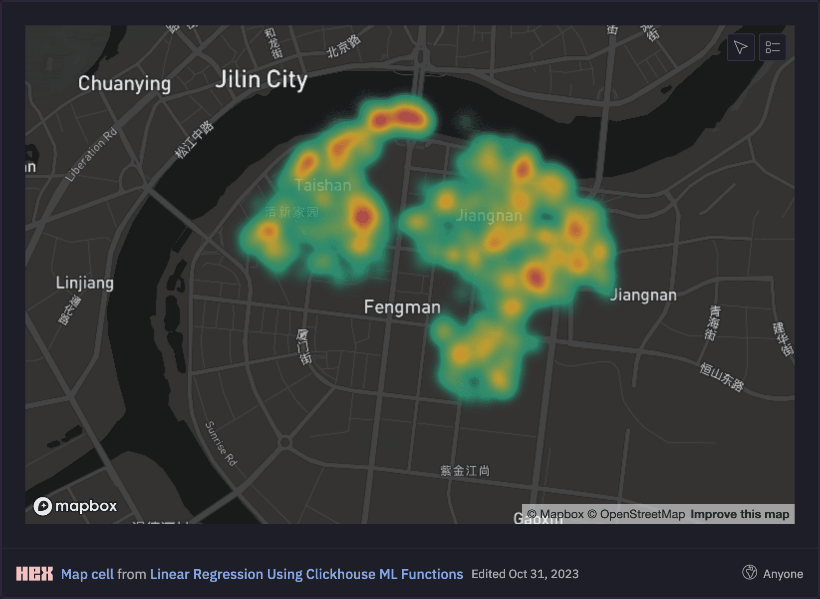
Using our Hex Notebook, we can easily render a heatmap of the delivery locations around Jilin, observing that more deliveries occur in central areas:
Our model will also take account of the pickup time as a second variable. Therefore, we will also visualise the distribution of the number of orders by pickup hour and can observe that most packages are collected at 8am in the morning.

Data preparation
Our model will predict the time elapsed between the pickup and delivery (in minutes) as a function of the distance between the pickup and the delivery locations (in meters) and of the pickup hour.
We use Clickhouse geoDistance function for calculating the distance between the pickup and the delivery locations given their coordinates (latitude and longitude), while we use Clickhouse date_diff function for calculating the time elapsed between pickup and delivery.
We also add to the dataset a randomly generated training index using randUniform function, which is equal to 1 for 80% of the data, which will be used for training, and equal to 0 for the remaining 20% of the data, which will be used for testing performance of the model.
CREATE TABLE deliveries_dataset (
        order_id UInt32,
        delivery_time Float64,
        delivery_distance Float64,
        Hour7 Float64,
        Hour8 Float64,
        Hour9 Float64,
        Hour10 Float64,
        Hour11 Float64,
        Hour12 Float64,
        Hour13 Float64,
        Hour14 Float64,
        Hour15 Float64,
        Hour16 Float64,
        training Float64
    )
ENGINE = MERGETREE
ORDER BY order_id
INSERT INTO deliveries_dataset
SELECT
    order_id,
    date_diff('minute', accept_gps_time, delivery_gps_time) as delivery_time,
    geoDistance(accept_gps_lng, accept_gps_lat, delivery_gps_lng, delivery_gps_lat) as delivery_distance,
    if(toHour(accept_gps_time) = 7, 1, 0) as Hour7,
    if(toHour(accept_gps_time) = 8, 1, 0) as Hour8,
    if(toHour(accept_gps_time) = 9, 1, 0) as Hour9,
    if(toHour(accept_gps_time) = 10, 1, 0) as Hour10,
    if(toHour(accept_gps_time) = 11, 1, 0) as Hour11,
    if(toHour(accept_gps_time) = 12, 1, 0) as Hour12,
    if(toHour(accept_gps_time) = 13, 1, 0) as Hour13,
    if(toHour(accept_gps_time) = 14, 1, 0) as Hour14,
    if(toHour(accept_gps_time) = 15, 1, 0) as Hour15,
    if(toHour(accept_gps_time) = 16, 1, 0) as Hour16,
    if(randUniform(0, 1) <= 0.8, 1, 0) as training
FROM
    deliveries
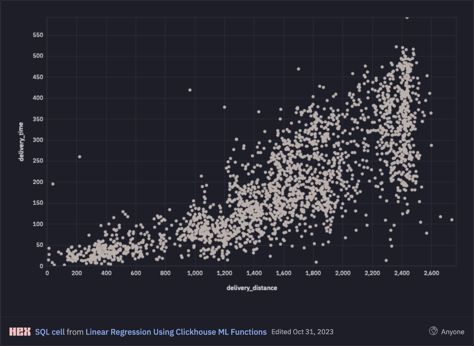
When visualised, delivery distance and delivery time are positively correlated with greater variance as journeys get longer. This is intuitively as we would expect as longer journeys become harder to predict.
Model training
We use Clickhouse's stochasticLinearRegression function for fitting the linear regression model based on the 80% of our dataset which contains training data.
Given that this function uses gradient descent, we scale the delivery distance (which is the only continuous feature) by subtracting the training set mean and dividing by the training set standard deviation. We take the logarithm of the target to make sure that the time to delivery predicted by the model is never negative.
CREATE VIEW deliveries_model AS WITH
    (SELECT avg(delivery_distance) FROM deliveries_dataset WHERE training = 1) AS loc,
    (SELECT stddevSamp(delivery_distance) FROM deliveries_dataset WHERE training = 1) AS scale
SELECT
    stochasticLinearRegressionState(0.1, 0.0001, 15, 'SGD')(
        log(delivery_time),
        assumeNotNull((delivery_distance - loc) / scale),
        Hour7,
        Hour8,
        Hour9,
        Hour10,
        Hour11,
        Hour12,
        Hour13,
        Hour14,
        Hour15,
        Hour16
    )  AS  STATE
FROM  deliveries_dataset WHERE training = 1
Model evaluation
We can now use the fitted model to make predictions for the remaining 20% of our dataset. We will do this by comparing the predicted delivery times with the actuals to calculate the accuracy of our model.
CREATE VIEW deliveries_results AS WITH
    (SELECT avg(delivery_distance) FROM deliveries_dataset WHERE training = 1) AS loc,
    (SELECT stddevSamp(delivery_distance) FROM deliveries_dataset WHERE training = 1) AS scale,
    (SELECT state from deliveries_model) AS model
SELECT
    toInt32(delivery_time) as ACTUAL,
    toInt32(exp(evalMLMethod(
        model,
        assumeNotNull((delivery_distance - loc) / scale),
        Hour7,
        Hour8,
        Hour9,
        Hour10,
        Hour11,
        Hour12,
        Hour13,
        Hour14,
        Hour15,
        Hour16
    ))) AS PREDICTED
FROM deliveries_dataset  WHERE training = 0
We now have a table of ACTUAL delivery times and PREDICTED delivery times for the 20% test portion of our dataset.
SELECT * FROM deliveries_results LIMIT 10

┌─ACTUAL─┬─PREDICTED─┐
│    410 │       370 │
│    101 │       122 │
│    361 │       214 │
│    189 │        69 │
│    122 │        92 │
│    454 │       365 │
│    155 │       354 │
│    323 │       334 │
│    145 │       153 │
│     17 │        20 │
└────────┴───────────┘

10 rows in set. Elapsed: 0.015 sec. Processed 9.17 thousand rows, 267.76 KB (619.10 thousand rows/s., 18.07 MB/s.)
Peak memory usage: 2.28 MiB.
We can also plot these visually as per below in our notebook:
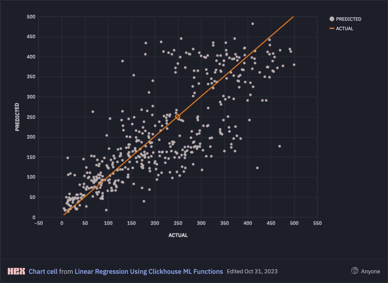
To explain the plot, if the model was performing perfectly, then we would expect PREDICTED and ACTUAL to match in every case, meaning that all points would line up on the orange curve. In reality, our model did have errors which we will now analyse.
Model performance
Looking at the visualisation above, we can see that our model performed relatively well for shorter journeys less than 120 minutes, but predictive accuracy begins to fall away for longer distance journeys as they become more complex and harder to predict.
This would be in line with our real-world experience whereby the longer and more arduous a journey is, the harder it is to predict.
More scientifically, we can evaluate the models performance by looking at the model's mean absolute error (MAE) and root mean squared error (RMSE). This gives us a value of approximately 1 hour across the entire dataset:
SELECT
    avg(abs(ACTUAL - PREDICTED)) AS MAE,
    sqrt(avg(pow(ACTUAL - PREDICTED, 2))) AS RMSE
FROM deliveries_results

┌───────────────MAE─┬──────────────RMSE─┐
│ 58.18494623655914 │ 78.10208373578114 │
└───────────────────┴───────────────────┘

1 row in set. Elapsed: 0.022 sec. Processed 9.17 thousand rows, 267.76 KB (407.90 thousand rows/s., 11.91 MB/s.)
Peak memory usage: 2.28 MiB.
If we limit this to just the shorter journeys with an ACTUAL of less than 2 hours (120 minutes), then we can see that our model performs better with an MAE and RMSE closer to 30 minutes:
SELECT
    avg(abs(ACTUAL - PREDICTED)) AS MAE,
    sqrt(avg(pow(ACTUAL - PREDICTED, 2))) AS RMSE
FROM deliveries_results
WHERE ACTUAL < 120

┌────────────────MAE─┬──────────────RMSE─┐
│ 29.681159420289855 │ 41.68671981213744 │
└────────────────────┴───────────────────┘

1 row in set. Elapsed: 0.014 sec. Processed 9.17 thousand rows, 267.76 KB (654.46 thousand rows/s., 19.11 MB/s.)
Peak memory usage: 2.35 MiB.
Conclusion
In this article we have demonstrated how we can use a simple linear regression function to predict output values based on 2 input variables.
The performance of the model was resasonable at shorter distances, but began to break down as the output variable became harder to predict. That said, we can see that a simple linear regression conducted entirely within ClickHouse and using only 2 variables does have some predictive capability and may perform better in other datasets and domains.
A notebook describing the full worked example can be found here.