Last month, we responded officially to the hugely successful 1 billion row challenge set by Gunnar Morling from Decodable. This challenge requires users to write a Java program to compute each city's minimum, average, and maximum temperatures from a text file containing 1 billion measurements. Our response to this challenge obviously used ClickHouse, which, despite being constrained by not being a specialized solution to the problem, posted a very respectable time of around 19 seconds using the exact hardware profile stipulated by the rules.
As any experienced ClickHouse user will know, 1 billion rows is quite small for ClickHouse, with users frequently performing aggregations over datasets in the trillions. So when the challenge was extended recently to 1 trillion rows by Dask, our curiosity was piqued.
In this blog post, we submit our attempt at querying the 1 trillion row dataset - completing the query in under 3 minutes for $0.56! While our original solution used moderate hardware, this larger challenge is a little trickier to perform on a laptop or machine equivalent to a small workstation.
Instead, we resort to using spot instances in AWS while aiming to find a compromise between cost and performance. Thanks to a largely linear pricing model from AWS, this is a straightforward task: we simply identify the best value instances in AWS that minimize the query performance. Using a Pulumi script, we can spin up a ClickHouse cluster, run the query, and shut down the resources - all for $0.56!
For those curious, if this data is loaded into a MergeTree, the query can be answered in 16 seconds! This incurs a load time, which we consider cheating, however :)
Dataset
The structure of the data provided by Dask is consistent with the original challenge, with a city and temperature column. As discussed in their original blog, data of this size requires a format offering better compression than the CSV used for the 1 billion row challenge. They, therefore, provide the data in Parquet format in the following requester-pays bucket, i.e., users downloading this will need to provide an access key for AWS and incur transfer charges.
s3://coiled-datasets-rp/1trc
However, provided we ensure our ClickHouse cluster is deployed in the same region as this bucket (us-east-1) we can avoid data transfer charges while also optimizing the network bandwidth and latency.
The full dataset consists of 2.4TiB of parquet files available as 100k files, each with 10m rows at around 23-24MiB.
Querying in place
Frequently accessed datasets can be loaded into an analytical database like ClickHouse for fast queries. But for infrequently used datasets, it’s sometimes helpful to leave them in a “lake house” like S3 and have the ability to run ad-hoc analytical queries on them in place. In the AWS ecosystem, users may be familiar with technologies such as Amazon Athena, which offers the ability to analyze data directly in Amazon S3 using standard SQL.
Technologies capable of querying both lakehouses and performing as a real-time analytical database can be considered real-time data warehouses.
ClickHouse offers both of these capabilities. For the purposes of our challenge, we only need to execute this query once. As noted in our 1 billion row challenge results, while the final query will be faster once the data has been loaded into ClickHouse, the actual load time will offset any benefit. We, therefore, utilize ClickHouse's s3 function to query the data "in-place".
SELECT
    count() as num_rows,
    uniqExact(_file) as num_files
FROM s3('https://coiled-datasets-rp.s3.us-east-1.amazonaws.com/1trc/measurements-*.parquet', 'AWS_ACCESS_KEY_ID', 'AWS_SECRET_ACCESS_KEY', headers('x-amz-request-payer' = 'requester'))

┌──────num_rows─┬─num_files─┐
│ 1000000000000 │    100000 │
└───────────────┴───────────┘
As a simple example, we can confirm the total number of rows and files with a simple query.
To access a requester-pays bucket, a header
'x-amz-request-payer' = 'requester'must be passed in any requests. This is achieved in the above call by passing the parameterheaders('x-amz-request-payer' = 'requester')to the s3 function.
A simple query
Our previous query for the 1 billion row challenge contained a few optimizations to minimize string formatting and to ensure the data was returned in the correct format. Thanks to the Parquet format, we aren’t required to do any string parsing. Our query is, therefore, a simple GROUP BY.
Minimizing AWS costs
To keep costs to an absolute minimum for our query, we can exploit AWS’ spot instances. These instance types allow you to use spare EC2 compute for which you can bid (a minimum spot price is set) through the AWS API. While potentially, these instances can be interrupted and reclaimed by AWS (e.g., if the spot price exceeds the bid), they come at up to a 90% discount. For current spot prices, we recommend this resource from Vantage.
These spot prices are not as linear for each instance type, unlike on-demand pricing. For example, at the time of writing, a c7g.xlarge with four vCPUs is $0.0693 per hour (> 50% cheaper than on demand), which is more than ½ the price of a c7g.2xlarge with eight cores at $0.1157. Long-term trends in supply and demand for EC2 spare capacity ultimately determine prices.
The next challenge was to minimize the time any instances were active. We need to:
- Claim our instances and wait for them to be available - usually around 30s
- Install ClickHouse and configure to form a cluster
- Run the query
- Immediately stop the instances.
This is a simplification of what needs to be done and doesn’t consider the need to configure supporting AWS resources, including a VPC, subnet, internet gateway, and an appropriate security group such that instances can communicate with each other.
To perform the AWS orchestration work and to configure a ClickHouse cluster, we chose Pulumi, principally because it allows the infrastructure provisioning code to be written in Python, making it very readable, as well as allowing all the work to be done in one tool. We've extended this with a Dynamic ResourceProvider to support querying the cluster once it's ready. This allows us to do all of the above work in a single script available here.
To reproduce these tests, users simply need to clone the above repository and modify the Pulumi stack configuration file shown below, specifying the region, zone, number of instances, and their respective type before running ./run.sh.
config:
 aws:region: us-east-1
 1trc:aws_zone: us-east-1d
 1trc:instance_type: "c7g.4xlarge"
 1trc:number_instances: 16
 # this must exist as a key-pair in AWS
 1trc:key_name: "<key-pair-name>"
 # change as needed
 1trc:cluster_password: "clickhouse_admin"
 # AMD ami (us-east-1)
 1trc:ami: "ami-05d47d29a4c2d19e1"
 # Intel AMI (us-east-1)
 # 1trc:ami: "ami-0c7217cdde317cfec"
 # query to run on the cluster
 1trc:query: "SELECT 1"
This script will invoke Pulumi up. This causes the instances to be provisioned and configured, executing the defined query as the final step. Once the query completes, Pulumi down is issued to teardown the infrastructure with a final timing reported.
We should stress that this script is in no way a substitute for proper provisioning code for a production ClickHouse cluster. We accepted some compromises given the ephemeral nature of the instances (less than 5 mins) but which would be severely limiting in a production cluster. Specifically:
- We don’t provision any storage as we query the data in place in S3.
- While access is limited to the IP from which the Pulumi code was run, the cluster is exposed over HTTP on port 8213 so we can run the required query. For the period the cluster is alive, this represents a minimal risk, but the lack of SSL would not be recommended for production environments. Our network settings for inter-instance communication are also too loose.
- The configuration of the cluster is extremely limited, with no consideration given to the need to modify, expand, or upgrade the cluster. Our ClickHouse configurations are also minimal and not customizable.
- Zero tests were performed, and no consideration is given to extensibility.
- We don’t handle potential spot interruptions that are always possible on AWS with spot instances. We also assume a homogeneous set of instance types (which is against AWS best practices) since this makes things easier to reason about and test.
While limited, the above script does allow us to spin up ClickHouse clusters cheaply, run a query, and destroy the infrastructure immediately. This ephemeral cluster deployment can be used to run queries that might otherwise be computationally out of reach for a laptop. For example, to run 32 instances of a c7g.4xlarge (16 cores, 32GiB RAM) for 5 minutes, we would pay approximately 0.2441 * (5/60) * 32 = $0.65 - ClickHouse can query a lot of data in S3 with this amount of resources!
Choosing an AWS instance type
Before performing any testing and query tuning we wanted to identify an instance type, mainly to avoid an exhaustive set of tests which would prove time consuming. We based this on simple reasoning with the aim of producing a competitive result without expending enormous resources to find the perfect hardware profile.
As a simple aggregation query, where the station has a relatively low cardinality (1000s), we suspected this query would be either CPU- or network-bound. As well as being cheaper per core than the Intel/AMD equivalents in AWS, ARM processors have performed well in our public benchmarks (see c7g) and testing. For example, if we consider the latest range of c7 instances for the size 4xlarge (16 vCPUs):
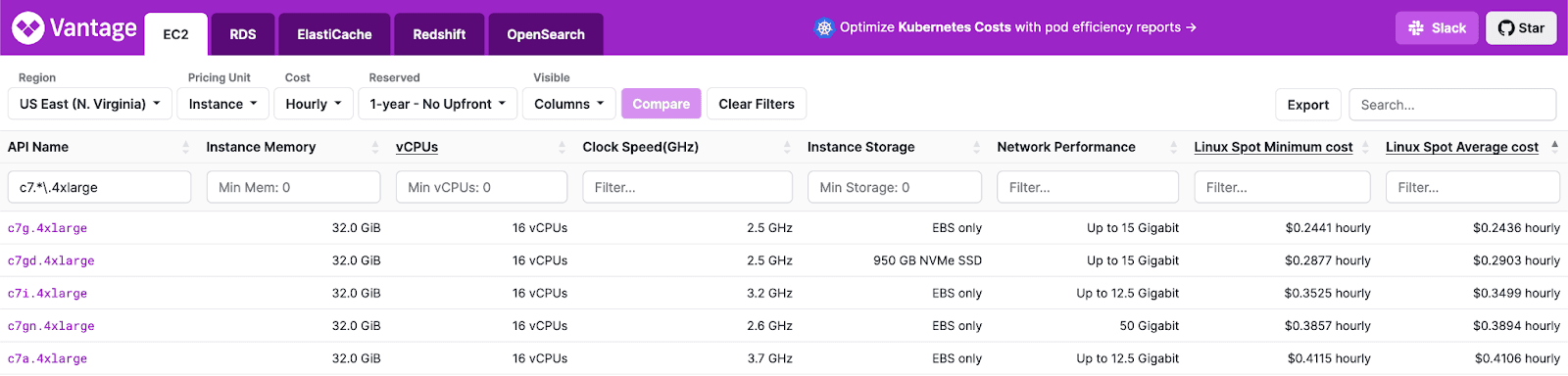
The c7g here represents our most cost-efficient option, especially since we don’t need the additional storage offered by the c7gd. The c7gn, while an identical ARM processor, does offer additional network bandwidth, which might be needed on very large instance sizes to avoid this becoming a bottleneck. This additional network bandwidth comes at a cost, however - 1.5x the spot cost!
Our decision on instance types, therefore, came down to the c7g or c7gn. Provided we scaled horizontally and didn’t use the larger instances where the network would likely be a bottleneck, the c7g made the most sense economically.
We also considered the slightly cheaper c6g instances. These were harder to obtain in our experience and have a slower network interface, but they may be worth considering in an exhaustive evaluation process.
As experienced ClickHouse users, we were fairly confident we could scale performance vertically. Our choice of which specific c7g instance thus came down to price per vCPU and availability. A quick analysis of c7g shows the larger instance types are generally more price-efficient on the spot market.
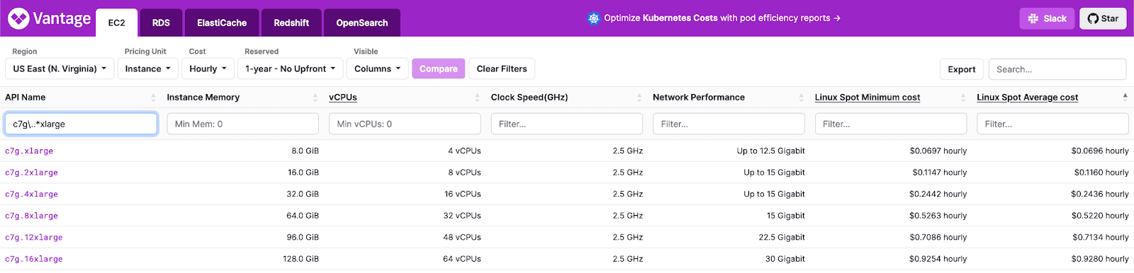
| Instance type | Avg price per hour ($) | vCPUs | Cost per vCPU |
|---|---|---|---|
| c7g.xlarge | 0.0696 | 4 | 0.0174 |
| c7g.2xlarge | 0.116 | 8 | 0.0145 |
| c7g.4xlarge | 0.2436 | 16 | 0.015225 |
| c7g.8xlarge | 0.522 | 32 | 0.0163125 |
| c7g.12xlarge | 0.7134 | 48 | 0.0148625 |
| c7g.16xlarge | 0.928 | 64 | 0.0145 |
These prices represent an average. Prices do vary per availability zone. For our final tests, we use the cheapest current zone. This can be established from the AWS console.
While the c7g.16xlarge represented the most cost-efficient choice, we struggled to obtain a significant number of these during testing - despite them appearing to have similar availability. We found the c7g.12xlarge to be easier to provision with minimal difference in the price.
Optimizing query settings
With the c7g.12xlarge selected as our instance type, we wanted to ensure query settings were optimal to minimize query runtime. For our performance test, we used a single instance and queried a subset of the data using the pattern measurements-1*.parquet. As shown below, this targets around 111 billion rows and delivers an initial response time of 454s.
SELECT station, min(measure), max(measure), round(avg(measure), 2)
FROM s3('https://coiled-datasets-rp.s3.us-east-1.amazonaws.com/1trc/measurements-1*.parquet', 'AWS_ACCESS_KEY_ID', 'AWS_SECRET_ACCESS_KEY', headers('x-amz-request-payer' = 'requester'))
GROUP BY station
ORDER BY station ASC
FORMAT `Null`

0 rows in set. Elapsed: 454.770 sec. Processed 111.11 billion rows, 279.18 GB (244.32 million rows/s., 613.88 MB/s.)
Peak memory usage: 476.72 MiB.
The above uses
FORMAT Nullso that results are not printed, and we can easily identify the actual query time. As the response is small, we consider this overhead negligible compared to the full query processing.
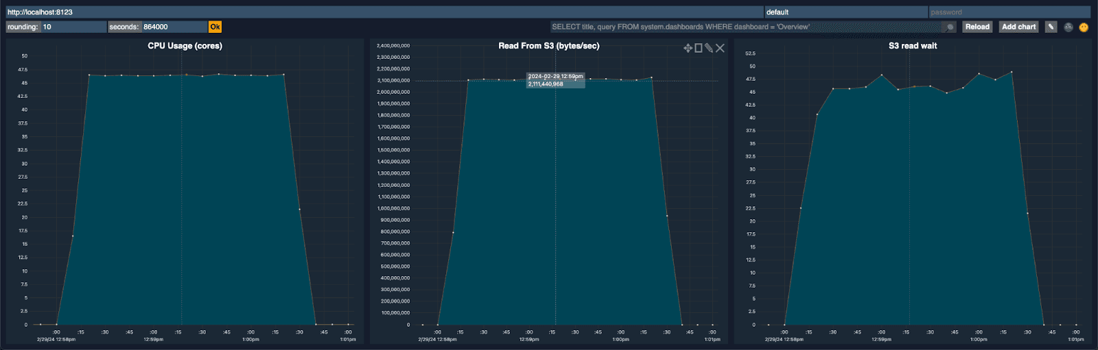
You can see immediately that at around 615 MB/s we were not network bound (instance supports 22.5Gbps). We evaluated the resource utilization for the cluster using the ClickHouse dashboard. Three immediate visualizations stood out here: the number of CPU cores used for the query, read performance from S3, and the S3 read wait time.
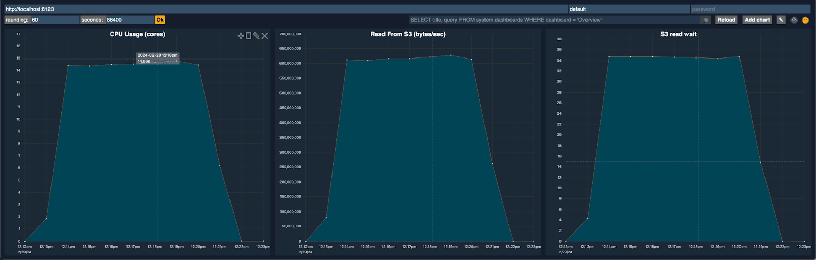
The number of CPU cores used for this query was around 14-15 (consistent with what the ClickHouse client reports during execution) and significantly less than the 48 available. Prior to any thread tuning, we spent some time evaluating why this might be the case. The S3 read wait time suggested we were issuing too many reads (this was confirmed with a query trace). A quick browse of our documentation states:
“For the s3 function and table, parallel downloading is determined by the values max_download_threads and max_download_buffer_size. Files will only be downloaded in parallel if their size is greater than the total buffer size combined across all threads. This is only available on versions > 22.3.1.”
The parquet files are around 25MB with the max_download_buffer_size default set to 10MiB. Given the simplicity of this query (it's just reading and doing a trivial aggregation), we knew we could safely increase this buffer size to 50 MB (max_download_buffer_size=52428800), with the aim of ensuring each file was downloaded by a single thread. This would reduce the time each thread spends making S3 calls and thus also lower the S3 wait time.
Increasing the buffer size to 50MiB:
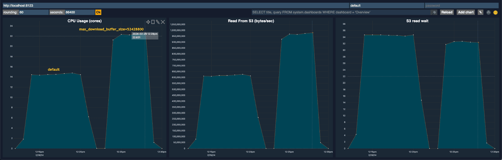
We can see this reduced our S3 read wait by about 20% while increasing our read throughput to over 920 MB/sec. With less time spent waiting, we utilize our threads more efficiently, increasing CPU utilization to around 23 cores. All of this has the effect of reducing our execution time from 486 seconds to 303s seconds.
0 rows in set. Elapsed: 303.462 sec. Processed 111.11 billion rows, 279.18 GB (366.14 million rows/s., 919.97 MB/s.)
Peak memory usage: 534.87 MiB.
After confirming that further increases in the buffer size yielded no benefit, as expected, and given that at 920MB/s, our instances are still definitely not network bound, we considered how we might further increase the CPU utilization.
By default most stages of this query will be run with 48 threads on each node as confirmed with an EXPLAIN PIPELINE:
EXPLAIN PIPELINE
SELECT
	station,
	min(measure),
	max(measure),
	round(avg(measure), 2)
FROM s3('https://coiled-datasets-rp.s3.us-east-1.amazonaws.com/1trc/measurements-1*.parquet', 'AWS_ACCESS_KEY_ID', 'AWS_SECRET_ACCESS_KEY', headers('x-amz-request-payer' = 'requester'))
GROUP BY station
ORDER BY station ASC

┌─explain─────────────────────────────────────┐
│ (Expression)                            	  │
│ ExpressionTransform                     	  │
│   (Sorting)                             	  │
│   MergingSortedTransform 48 → 1         	  │
│ 	MergeSortingTransform × 48          	  │
│   	LimitsCheckingTransform × 48      	  │
│     	PartialSortingTransform × 48    	  │
│       	(Expression)                  	  │
│       	ExpressionTransform × 48      	  │
│         	(Aggregating)               	  │
│         	Resize 48 → 48              	  │
│           	AggregatingTransform × 48 	  │
│             	StrictResize 48 → 48    	  │
│               	(Expression)          	  │
│               	ExpressionTransform × 48  │
│                 	(ReadFromStorageS3Step)   │
│                 	S3 × 48 0 → 1       	  │
└─────────────────────────────────────────────┘

17 rows in set. Elapsed: 0.305 sec.
This defaults to the number of vCPUs per node by default and represents a sensible default for most queries. In our case, given the read-intensive nature of the task, increasing this made sense.
Ideally we would like to be able to increase just the number of download threads in this test. Currently, this isn’t available as a setting in ClickHouse, but is something we’re considering.
While we didn’t perform exhaustive testing, some simple tests showed the benefit of increasing the max_threads to 128:
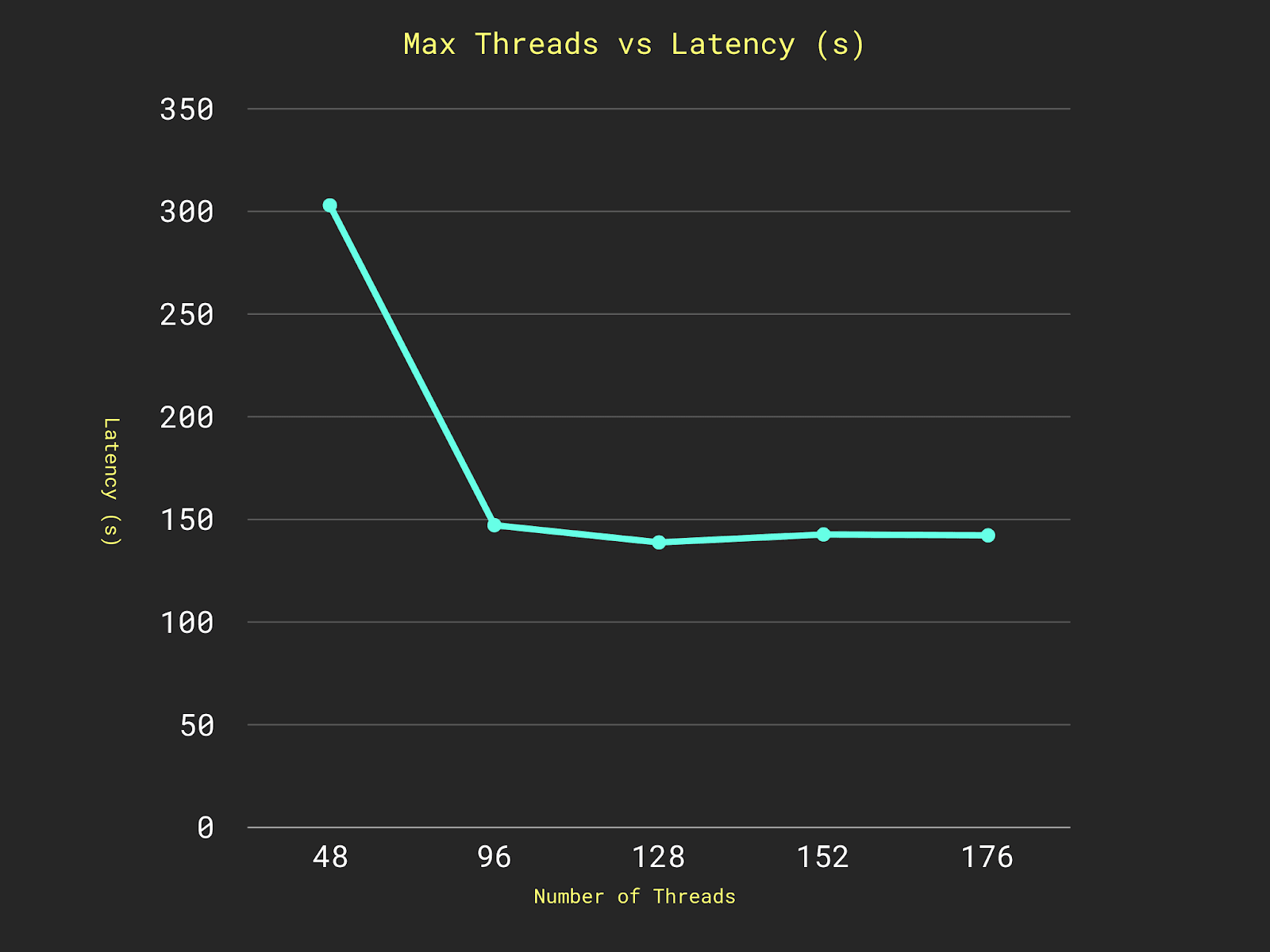
The above represents the average from 3 executions.
This also delivered a decent improvement, reducing the total runtime to 138 seconds.
0 rows in set. Elapsed: 138.820 sec. Processed 111.11 billion rows, 279.18 GB (800.39 million rows/s., 2.01 GB/s.)
Peak memory usage: 1.36 GiB.
Returning to our advanced dashboard, we can see this increased our read throughput to around 2 GiB/s (still not network bound) with 46 of the 48 cores utilized. Further increases in the max_threads beyond 128 resulted in CPU contention and CPU wait time - reducing overall throughput.
At this point, we were content that we were CPU bound and did not believe further tuning would deliver significant gains; our final query time was 138 seconds or around 2 minutes to query all 111 billion rows.
A single instance is obviously not sufficient to give us a reasonable runtime on a dataset almost 10x the size. However, confident our individual c7g.12xlarge will not be network bound, and with sensible settings for our query, we scale horizontally and tackle our larger 1 trillion row problem.
When we run our query across a cluster, these same settings can be passed to each node, along with a subset of the data to process, thus optimizing the performance of each.
Using a cluster
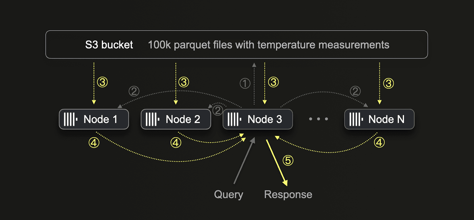
To query a cluster and use all nodes, we had to change our query a little, using the s3Cluster rather than the s3 function. This allows us to use all nodes in our cluster to process the query.
Unlike the standard s3 function, which executes the query on the receiving node only, this function ① first performs a listing of the bucket. The coordinating node uses this list to ② send files to be processed to every node in the cluster, thus allowing the work to be parallelized ③. The coordinating node then ④ collates intermediate results from each of the nodes in the cluster to ⑤ provide the final response. We visualize this below:
Our final query:
SELECT station,
	min(measure),
	max(measure),
	round(avg(measure), 2)
FROM s3Cluster('default', 'https://coiled-datasets-rp.s3.us-east-1.amazonaws.com/1trc/measurements-*.parquet', 'AWS_ACCESS_KEY_ID', 'AWS_SECRET_ACCESS_KEY', headers('x-amz-request-payer' = 'requester'))
GROUP BY station
ORDER BY station ASC
FORMAT `Null`
SETTINGS max_download_buffer_size = 52428800, max_threads = 110
In our example above, as in all ClickHouse Cloud clusters, we name our cluster 'default'.
Final timing and costs
While the query time should reduce linearly with the number of instances we deploy, thus keeping cost constant, we were also restricted as to how many instances we could realistically provision. AWS generally recommends mixed instance types and EC2 scaling groups instead of our homogenous approach to scaling. Our current script also restricts us to a single availability zone (although this is an obvious improvement, it complicates the code a little). A little testing revealed eight instances could be reliably obtained, giving us a total of 384 vCPUs. Our final configuration was thus:
config:
  aws:region: us-east-1
  1trc:aws_zone: us-east-1b
  1trc:instance_type: "c7g.12xlarge"
  1trc:number_instances: 8
  1trc:key_name: "dalem"
  1trc:cluster_password: "a_super_password"
  # AMD ami (us-east-1)
  1trc:ami: "ami-05d47d29a4c2d19e1"
  1trc:query: "SELECT station, min(measure), max(measure), round(avg(measure), 2) FROM s3Cluster('default','https://coiled-datasets-rp.s3.us-east-1.amazonaws.com/1trc/measurements-*.parquet', 'AWS_ACCESS_KEY_ID', 'AWS_SECRET_ACCESS_KEY', headers('x-amz-request-payer' = 'requester')) GROUP BY station ORDER BY station ASC SETTINGS max_download_buffer_size = 52428800, max_threads=128"
Note we use us-east-1b as our availability zone. At the time of writing, this was the cheapest zone at 0.7162 per instance per hour (a 58.84% saving over on-demand instances).
With our optimal settings, we can run our run script:
./run.sh

(venv) dalemcdiarmid@PY aws-starter % ./run.sh
Updating (dev)

View in Browser (Ctrl+O): https://app.pulumi.com/clickhouse/aws-starter/dev/updates/88

 	Type                           	Name                         	Status          	Info
 +   ├─ aws:ec2:Instance            	1trc_node_4                  	created (17s)
 +   ├─ aws:ec2:Instance            	1trc_node_2                  	created (17s)
 +   ├─ aws:ec2:Instance            	1trc_node_7                  	created (18s)

…

 +   └─ pulumi-python:dynamic:Resource  1trc-clickhouse-query        	created (181s)

Diagnostics:
  pulumi:pulumi:Stack (aws-starter-dev):
	info: checking cluster is ready...
	info: cluster is ready!
	info: running query...
	info: query took 178.94s ← query time!

Resources:
	+ 80 created

Duration: 5m10s ← startup time + query time!

…

Destroying (dev)

View in Browser (Ctrl+O): https://app.pulumi.com/clickhouse/aws-starter/dev/updates/89

 	Type                   	Name                   	Status
 	pulumi:pulumi:Stack    	aws-starter-dev
 -   ├─ command:remote:Command  restart_node_3_clickhouse  deleting (26s)...
 -   ├─ command:remote:Command  restart_node_2_clickhouse  deleting (26s)...
 -   ├─ command:remote:Command  restart_node_4_clickhouse  deleting (26s)...
 -   ├─ command:remote:Command  restart_node_5_clickhouse  deleting (26s)...

…

Resources:
	- 80 deleted

Duration: 2m58s ← time to remove resources

The resources in the stack have been deleted, but the history and configuration associated with the stack are still maintained.
If you want to remove the stack completely, run `pulumi stack rm dev`.
Total time: 499 seconds
From the output, we can see our query completed in under 180 seconds or 3 minutes. However, our cluster took around 2 mins 10 seconds to provision and be available to query before taking a further 3 minutes to terminate. Our total runtime was, therefore, 499 seconds.
We can use thus to compute our final cost.
Cost per instance: $0.7162
Number of instances: 8
Time active: 499s
Cost: (499/3600) * 8 * 0.7162 = $0.79
This represents an estimate of the cost only. There are several factors that might cause the incurred cost to be different - mainly that all instances are not active for the full 499 seconds. By subscribing to the Spot Instance data feed an exact cost can be obtained. This sends costs associated with spot instances to an S3 bucket for later retrieval. Examining the statistics for our test run, we can see the actual incurred costs for each instance:
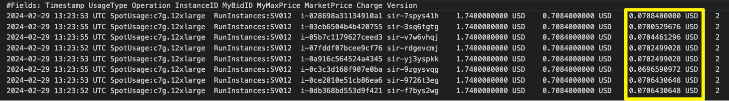
Adding these up gives our total price for querying 1 trillion rows:
(0.0708400000+0.0700529676+0.0704461296+0.0702499028+0.0702499028+0.0696590972+0.0706430648+0.0706430648) = $0.56
Final thoughts
It's worth noting that while more instances will reduce the query time, they will take longer to provision, potentially incurring more costs. It, therefore, makes sense to scale vertically before horizontally as this dominates the run time. However, should you be running multiple queries, this time is negated since it's a one-off cost!
As someone who doesn't claim to be an expert in Pulumi, I also suspect the provisioning (and termination code) could be improved to minimize the startup and shutdown timings. We, as ever, welcome contributions!
In developing this approach, we haven't diligently adhered to AWS best practices with respect to Spot instances. An improved version of this code could use heterogeneous instance types and even exploit EC2 Auto Scaling groups to allow the user to simply specify the number of cores required! An AMI with ClickHouse pre-installed could further reduce startup times, and flexibility in AWS zones would likely allow easier scaling.
An astute reader will have noticed we didn't provision our spot instances with a bid. We simply accepted the spot price for the current hour. If you really want to save a few cents, there is room to lower this price further!
With MergeTree
Finally, we were curious as to how fast this data could be queried in a MergeTree table engine. While loading the data into a table also takes some time (it was 385s on a 300 core ClickHouse Cloud cluster), querying the resulting table with a full scan takes only 16.5s and is overwhelmingly faster than any results of querying parquet files (same cluster achieves the query in 48s)! Note that such a cluster can easily be deployed through the ClickHouse Cloud API, used to run the query, and then be immediately terminated. Credit Alexey Milovidov for these timings.
Conclusion
Expanding on the billion-row challenge, we’ve shown how ClickHouse allows an even larger 1 trillion dataset to be queried in under 3 minutes for $0.56!!
We welcome suggestions or alternatives to query this dataset faster and more cost-efficiently.